A revised averaging method and general forms of approximate solution for nonlinear oscillator with only polynomial-type displacement nonlinearity

Shen, Yongjun; Zhao, Yongxiang; Yang, Shaopu; Xing, Haijun

Journal of Vibroengineering

Browse Journal

Submit article

Published: 30 June 2014

Check for updates

A revised averaging method and general forms of approximate solution for nonlinear oscillator with only polynomial-type displacement nonlinearity

Yongjun Shen¹

Yongxiang Zhao²

Shaopu Yang³

Haijun Xing⁴

^{1, 2, 3, 4}Department of Mechanical Engineering, Shijiazhuang Tiedao University, Shijiazhuang, 050043, China

Corresponding Author:

Yongjun Shen

Cite the article Download PDF

Downloads 1196

Abstract

In this paper a revised averaging method is presented, that does not need the detuning factor in the solving procedure. Comparison with the traditional averaging method shows that it has the similar solving procedure and the same result as the primary resonance of the traditional averaging method. Then the nonlinear oscillator with only polynomial-type displacement nonlinearity is studied, and the general forms of the first-order approximate solution by this revised averaging method, and by the traditional averaging method for the super-harmonic resonance and sub-harmonic resonance are established. At last, the Duffing oscillator is investigated as an example, and the comparison of the analytical and numerical results proves the validity and simplicity of the presented method.

1. Introduction

Averaging method is an effective analytical method for the approximate solution of the weakly nonlinear system. Since its presentation [1, 2], averaging method had been revised and improved to process a lot of nonlinear problems, and some relevant advances were summarized in the monographs [1-4].

Averaging method has been applied in a great deal theoretic and engineering problems extensively [5-13]. For example, Wang and Hu [5] reduced the delay differential equation of infinite dimensional to an ordinary differential equation by averaging method. Roy [6] developed the averaging method to find the periodic solutions of strongly nonlinear oscillators with harmonic excitations. Chatterjee [7] improved the averaging method based on harmonic balance, where the closed form solutions to the unperturbed problem were not needed, so as to research some strongly nonlinear system. Kumar and Datta [8] used the stochastic averaging technique to research the probability density function of the response for strongly nonlinear system subject to both multiplicative and additive random excitations. Ji and Hansen [9] constructed a valid asymptotic expansion solution of a nonlinear oscillator composed of a weakly nonlinear and a linear differential equation based on the averaging method and the continuity condition. Then they [10] extended this strategy to an approximate solution for the super-harmonic resonance of a periodically excited nonlinear oscillator with a piecewise nonlinearity, and the validity of the developed analysis was confirmed by comparing the approximate solutions with the results of direct numerical integration of the original equation. Yang, Tang, Chen and Lim [11] applied the averaging method to analyze the instability phenomena caused by sub-harmonic and combination resonance of transverse parametric vibrations of an axially accelerating tensioned Timoshenko beam on simple supports. Li, Ji and Hansen [12] studied a system composed of two Van der Pol oscillators with delayed position and velocity coupling by the averaging method, where the stability and the number of periodic solutions in 1:1 internal resonance were researched. Yang and Chen [13] investigated the parametrical vibration of a nonlinear oscillator with Davidenkov’s hysteretic nonlinearity by the averaging method and singularity theory, and the universal unfolding was also obtained.

In the above researches, the averaging method were generally used to obtain the approximate solution according to the relationship between the excitation frequency and the natural frequency, so as to induce different responses, such as the primary resonance, sub-harmonic resonance and super-harmonic resonance, etc. In this paper, we revise the traditional averaging method, and find that the revised averaging method could obtain the entirely same form as the primary resonance of the traditional averaging method when researching the first-order approximate solution. And the presented method does not need to introduce the detuning factor as the traditional averaging method. Then the general forms of the approximate solutions of nonlinear system with only polynomial-type displacement nonlinearity are established, which may make the research on this kind of nonlinear system more convenient. At last the validity of the presented method is proved by comparison of the approximate solution and the numerical one of the Duffing oscillator.

2. The revised averaging method

The nonlinear system considered here is:

1

\ddot{x} (t) + ω_{0}^{2} x (t) = p (x, \dot{x}) + F c o s (ω t),

where $ω_{0}$ is the natural frequency, $p (x, \dot{x})$ includes linear damping force, nonlinear damping force and nonlinear restoring force, $F$ and $ω$ is the amplitude and frequency of external excitation respectively.

In traditional averaging method and other perturbation-based methods [14-15], such as multi-scale method, KBM method, it is necessary to consider that whether the excitation frequency $ω$ is close to the natural frequency, associated with the multiple or fraction of the natural frequency $ω_{0}$ . Hence the solving procedure could be divided into some cases such as the primary resonance, secondary resonance including super-harmonic resonance and sub-harmonic resonance, etc. And some detuning factors should be introduced in the traditional averaging method.

Here we present the revised averaging method, where it is unnecessary to distinguish the above cases and introduce the detuning factor.

Letting the solution of Eq. (1) as:

2a

x = a c o s (ω t + θ),

and

2b

\dot{x} = - a ω s i n (ω t + θ) .

By differentiating Eq. (2a) to $t$ , one could obtain:

3

\dot{x} = \dot{a} c o s ϕ - a (ω + \dot{θ}) s i n ϕ,

where $ϕ = ω t + θ$ . Combined with Eq. (2b), it yields:

4

\dot{a} c o s ϕ - a \dot{θ} s i n ϕ = 0 .

By differentiating Eq. (2b) to $t$ , one could obtain:

5

\ddot{x} = - \dot{a} ω s i n ϕ - a ω (ω + \dot{θ}) c o s ϕ .

Combined Eq. (5) with Eq. (1), it will yield:

6

\dot{a} s i n ϕ + a \dot{θ} c o s ϕ = - \frac{1}{ω} [F c o s (ϕ - θ) + p (a c o s ϕ, - a ω s i n ϕ) + a (ω^{2} - ω_{0}^{2}) c o s ϕ] .

From Eq. (4) and Eq. (6), and by solving the system of equations with $\dot{a}$ and $\dot{θ}$ as unknowns, one could get:

7a

\dot{a} = - \frac{1}{ω} P (a, θ) s i n ϕ,

and

7b

a \dot{θ} = - \frac{1}{ω} P (a, θ) c o s ϕ,

where $P (a, θ) = F c o s (ϕ - θ) + p (a c o s ϕ, - a ω s i n ϕ) + a (ω^{2} - ω_{0}^{2}) c o s ϕ$ .

Applying the averaging procedure to Eq. (7) in a periodic $T$ (here $T = 2 π$ ), that means:

8a

\dot{a} = - \frac{1}{T ω} \int_{0}^{T} P (a, θ) s i n ϕ d ϕ,

8b

\dot{θ} = - \frac{1}{a T ω} \int_{0}^{T} P (a, θ) c o s ϕ d ϕ .

Moreover, one could obtain the simpler form as:

9a

\dot{a} = - \frac{F}{2 ω} s i n θ - \frac{1}{T ω} \int_{0}^{T} p (a, θ) s i n ϕ d ϕ,

9b

\dot{θ} = - \frac{F}{2 a ω} c o s θ - \frac{ω^{2} - ω_{0}^{2}}{2 ω} - \frac{1}{a T ω} \int_{0}^{T} p (a, θ) c o s ϕ d ϕ .

3. The traditional averaging method

In traditional averaging method, one must consider the approximation degree of the excitation frequency $ω$ to the natural frequency $ω_{0}$ , associated with the multiple or the fraction of natural frequency $ω_{0}$ .

3.1. Primary resonance

This case means the excitation frequency $ω$ is close to the natural frequency $ω_{0}$ . In order to illustrate the approximation degree, one should introduce:

10

ω^{2} = ω_{0}^{2} + ε σ,

where $ε$ is a small dimensionless parameter and $σ$ is the detuning factor. The nonlinear restoring force and the damping force $p (x, \dot{x})$ , the amplitude of excitation force $F$ should also be re-scaled as:

11

p (x, \dot{x}) = ε p_{1} (x, \dot{x}), F = ε f .

Then Eq. (1) could be transformed into:

12

\ddot{x} (t) + ω^{2} x (t) = ε p_{1} (x, \dot{x}) + ε σ x + ε f c o s (ω t) .

Letting the solution has the form as Eq. (2a) and Eq. (2b), and after the similar deducing procedure, one could obtain:

13a

\dot{a} = - \frac{1}{ω} Q (x, \dot{x}, t) s i n ϕ,

13b

a \dot{θ} = - \frac{1}{ω} Q (x, \dot{x}, t) c o s ϕ,

where $Q (x, \dot{x}, t) = ε [p_{1} (x, \dot{x}) + σ a c o s ϕ + f c o s (ϕ - θ)]$ .

Averaging the right-hand side of Eq. (13) in a periodic $T$ (here $T = 2 π$ ), it would be:

14a

\dot{a} = - \frac{ε f}{2 ω} s i n θ - \frac{ε}{T ω} \int_{0}^{T} p_{1} (a, θ) s i n ϕ d ϕ,

14b

\dot{θ} = - \frac{ε f}{2 a ω} c o s θ - \frac{ε σ}{2 ω} - \frac{ε}{a T ω} \int_{0}^{T} p_{1} (a, θ) c o s ϕ d ϕ .

Based on the scale relationship shown in Eq. (11), it could be concluded that Eq. (13) and Eq. (14) are entirely the same as Eq. (7) and Eq. (9). Accordingly, the revised averaging method is totally equal to the primary resonance of the traditional averaging method. Nevertheless, it is unnecessary to introduce the detuning factor in the revised method as the traditional averaging method, which could make the deducing procedure much simpler.

3.2. Super-harmonic resonance

In traditional averaging method, super-harmonic resonance means that the multiple of the excitation frequency is close to the natural frequency, i.e. $ω_{0} \approx n ω$ , where $n$ is a natural number unequal to 1. In order to illustrate the approximation degree of $n ω$ to $ω_{0}$ , introducing:

15

{(n ω)}^{2} = ω_{0}^{2} + ε σ,

where $ε$ is a small dimensionless parameter and $σ$ is the detuning factor. The nonlinear restoring force and the damping force $p (x, \dot{x})$ should be rescaled as:

16

p (x, \dot{x}) = ε p_{1} (x, \dot{x}),

that yields:

17

\ddot{x} (t) + {(n ω)}^{2} x (t) = ε p_{1} (x, \dot{x}) + ε σ x + F c o s (ω t) .

The solution should be as:

18

x = a c o s ϕ + B c o s (ω t),

\dot{x} = - a n ω s i n ϕ - B ω s i n (ω t),

where:

ϕ = n ω t + θ, B = \frac{F}{(n^{2} - 1) ω^{2}} .

Based on the standard procedure of averaging method, one can obtain:

19a

\dot{a} = - \frac{ε}{n ω} P (a, ϕ) s i n ϕ,

19b

a \dot{θ} = - \frac{ε}{n ω} P (a, ϕ) c o s ϕ,

where $P (a, ϕ) = p_{1} (a, ϕ) + σ [a c o s ϕ + B c o s [(ϕ - θ) / n]]$ .

Averaging the right-hand side of Eq. (19) in a periodic $T$ (here $T = 2 n π$ ), it would be:

20a

\dot{a} = - \frac{ε}{T n ω} \int_{0}^{T} P (a, ϕ) s i n ϕ d ϕ,

20b

\dot{θ} = - \frac{ε}{T a n ω} \int_{0}^{T} P (a, ϕ) c o s ϕ d ϕ,

that could be simplified as:

21a

\dot{a} = - \frac{ε}{T n ω} \int_{0}^{T} p_{1} (a, ϕ) s i n ϕ d ϕ,

21b

\dot{θ} = - \frac{ε σ}{2 n ω} - \frac{ε}{T a n ω} \int_{0}^{T} p_{1} (a, ϕ) c o s ϕ d ϕ .

3.3. Sub-harmonic resonance

In traditional averaging method, sub-harmonic resonance means that the fraction of the excitation frequency is close to the natural frequency, i.e. $ω_{0} \approx ω / n$ , where $n$ is a natural number unequal to 1. In order to illustrate the approximation degree, introducing:

22

{(\frac{ω}{n})}^{2} = ω_{0}^{2} + ε σ,

where $ε$ is a small dimensionless parameter and $σ$ is the detuning factor. The nonlinear restoring force and the damping force $p (x, \dot{x})$ should be rescaled as:

23

p (x, \dot{x}) = ε p_{1} (x, \dot{x}),

that yields:

24

\ddot{x} (t) + {(\frac{ω}{n})}^{2} x (t) = ε p_{1} (x, \dot{x}) + ε σ x + F c o s (ω t) .

The solution should be as:

25

x = a c o s ϕ + B c o s (ω t),

\dot{x} = - \frac{a ω}{n} s i n ϕ - B ω s i n (ω t),

where:

ϕ = \frac{ω}{n} t + θ, B = \frac{n^{2} F}{(1 - n^{2}) ω^{2}} .

Based on the standard procedure of averaging method, one can obtain:

26a

\dot{a} = - \frac{ε n}{ω} P (a, ϕ) s i n ϕ,

26b

a \dot{θ} = - \frac{ε n}{ω} P (a, ϕ) c o s ϕ,

where $P (a, ϕ) = p_{1} (a, ϕ) + σ [a c o s ϕ + B c o s [n (ϕ - θ)]]$ .

Averaging the right-hand side of Eq. (26) in a periodic $T$ (here $T = 2 π$ ), it would be:

27a

\dot{a} = - \frac{ε n}{T ω} \int_{0}^{T} P (a, ϕ) s i n ϕ d ϕ,

27b

\dot{θ} = - \frac{ε n}{T a ω} \int_{0}^{T} P (a, ϕ) c o s ϕ d ϕ,

that could be simplified as:

28a

\dot{a} = - \frac{ε n}{T ω} \int_{0}^{T} p_{1} (a, ϕ) s i n ϕ d ϕ,

28b

\dot{θ} = - \frac{ε n σ}{2 ω} - \frac{ε n}{T a ω} \int_{0}^{T} p_{1} (a, ϕ) c o s ϕ d ϕ .

4. The general solution of nonlinear system with only polynomial-type displacement nonlinearity

In this section we consider a kind of nonlinear system, where the nonlinear part is only composed of polynomial-type nonlinear restoring force. That means:

29

p (x, \dot{x}) = - c \dot{x} - α x^{n} .

4.1. The revised averaging method

From Eq. (29), one could obtain:

30

p (a, θ) = c a ω s i n ϕ - α a^{n} {c o s}^{n} ϕ .

In order to obtain the explicit form for Eq. (9), we introduce the expansion forms for the even and odd powers of trigonometric function shown as page 28 in [16] or page 80-82 in [17]:

31

{c o s}^{2 l} β = \frac{1}{2^{2 l - 1}} [\sum_{k = 0}^{l - 1} C_{2 l}^{k} \cos (2 l - 2 k) β + \frac{1}{2} C_{2 l}^{l}],

{c o s}^{2 l + 1} β = \frac{1}{2^{2 l}} [\sum_{k = 0}^{l} C_{2 l + 1}^{k} \cos (2 l - 2 k + 1) β],

where $l$ is natural number, $C_{2 l}^{k} = (2 l)! / k! (2 l - k)!$ is the binominal coefficient ( $0! = 1$ ).

Based on Eq. (31) and the orthogonality of trigonometric function, the integral in Eq. (9a) is:

32

\int_{0}^{2 π} p (a, θ) s i n ϕ d ϕ = \int_{0}^{2 π} (c a ω s i n ϕ - α a^{n} {c o s}^{n} ϕ) s i n ϕ d ϕ = c a ω π .

The integral in Eq. (9b) is:

33

\int_{0}^{2 π} p (a, θ) c o s ϕ d ϕ = \int_{0}^{2 π} (c a ω s i n ϕ - α a^{n} {c o s}^{n} ϕ) c o s ϕ d ϕ = 0,

when $n$ is even, and:

34

\int_{0}^{2 π} (c a ω s i n ϕ - α a^{n} {c o s}^{n} ϕ) c o s ϕ d ϕ = - \frac{C_{2 l}^{l} a^{n} α π}{2^{n}},

when $n$ is odd (supposing $n = 2 l - 1$ ).

Accordingly, when the nonlinear part is only composed of polynomial-type nonlinear restoring force, Eq. (9a) and Eq. (14a) could be as:

35a

\dot{a} = - \frac{F}{2 ω} s i n θ - \frac{c a}{2},

and Eq. (9b) and Eq. (14b) could be as:

35b

\dot{θ} = \{\begin{array}{l} - \frac{F}{2 a ω} c o s θ - \frac{ω^{2} - ω_{0}^{2}}{2 ω}, & when n is even, \\ - \frac{F}{2 a ω} c o s θ - \frac{ω^{2} - ω_{0}^{2}}{2 ω} + \frac{α a^{n - 1} C_{2 l}^{l}}{2^{n + 1} ω}, & when n is odd and n = 2 l - 1 . \end{array}

4.2. The super-harmonic resonance

From Eq. (29), one could obtain:

36

p_{1} (a, θ) = c [a n ω s i n ϕ + B ω s i n (ω t)] - α {[a c o s ϕ + B c o s (ω t)]}^{n} .

In order to compute the integral in Eq. (21), the binomial theorem is adopted:

37

{(a_{1} + a_{2})}^{n} = \sum_{k = 0}^{n} C_{n}^{k} a_{1}^{n - k} a_{2}^{k},

where $a_{1}$ , $a_{2}$ is complex number and $C_{n}^{k}$ is the binomial coefficient.

Based on the aforementioned the expansion form for the even and odd powers of trigonometric function and the orthogonality of trigonometric function, the integral in Eq. (21a) is:

38

\int_{0}^{2 n π} p_{1} (a, ϕ) s i n ϕ d ϕ = c a n^{2} ω π - \frac{α n B^{n} π}{2^{n - 1}} s i n θ .

The integral in Eq. (21b) is:

39

\int_{0}^{2 n π} p_{1} (a, ϕ) c o s ϕ d ϕ = - \frac{α n B^{n} π}{2^{n - 1}} c o s θ,

when $n$ is even, and:

40

\int_{0}^{2 n π} p_{1} (a, ϕ) c o s ϕ d ϕ = - \frac{n π α a^{n} C_{2 l}^{l}}{2^{n}} - \frac{α n π}{2^{n}} \sum_{l_{2} = 1}^{l - 1} a^{n - 2 l_{2}} B^{2 l_{2}} C_{n}^{2 l_{2}} C_{n - 2 l_{2} + 1}^{l - l_{2}} C_{2 l_{2}}^{l_{2}}

- \frac{n π α B^{n}}{2^{n - 1}} c o s θ,

when $n$ is odd (supposing $n = 2 l - 1$ ).

Accordingly, Eq. (21) should be as:

41a

\dot{a} = - \frac{ε c a}{2} + \frac{ε α B^{n}}{2^{n} n ω} s i n θ,

41b

\dot{θ} = \{\begin{array}{l} - \frac{ε σ}{2 n ω} + \frac{ε α B^{n}}{2^{n} a n ω} c o s θ, & when n is even, \\ - \frac{ε σ}{2 n ω} + \frac{ε α}{2^{n + 1} a n ω} (a^{n} C_{2 l}^{l} + 2 B^{n} c o s θ + \sum_{l_{2} = 1}^{l - 1} a^{n - 2 l_{2}} B^{2 l_{2}} C_{n}^{2 l_{2}} C_{n - 2 l_{2} + 1}^{l - l_{2}} C_{2 l_{2}}^{l_{2}}), & when n is odd . \end{array}

4.3. The sub-harmonic resonance

From Eq. (29), one could obtain:

42

p_{1} (a, θ) = c [\frac{a ω}{n} s i n ϕ + B ω s i n (ω t)] - α {[a c o s ϕ + B c o s (ω t)]}^{n} .

Similarly as the super-harmonic resonance, the integral in Eq. (28a) is:

43

\int_{0}^{2 π} p_{1} (a, ϕ) s i n ϕ d ϕ = \frac{c a π ω}{n} - \frac{n α π a^{n - 1} B}{2^{n - 1}} s i n (n θ) .

The integral in Eq. (28b) is:

44

\int_{0}^{2 π} p_{1} (a, ϕ) c o s ϕ d ϕ = - \frac{n α B π a^{n - 1}}{2^{n - 1}} c o s (n θ),

when $n$ is even, and:

45

\int_{0}^{2 π} p_{1} (a, ϕ) c o s ϕ d ϕ = - \frac{π α a^{n} C_{2 l}^{l}}{2^{n}} - \frac{α π}{2^{n}} \sum_{l_{2} = 1}^{l - 1} a^{n - 2 l_{2}} B^{2 l_{2}} C_{n}^{2 l_{2}} C_{n - 2 l_{2} + 1}^{l - l_{2}} C_{2 l_{2}}^{l_{2}} - \frac{n π α a^{n - 1} B}{2^{n - 1}} c o s (n θ),

when $n$ is odd.

Accordingly, Eq. (28) should be as:

46a

\dot{a} = - \frac{ε c a}{2} + \frac{ε α n^{2} a^{n - 1} B}{2^{n} ω} s i n (n θ),

\dot{θ} = - \frac{ε n σ}{2 ω} + \frac{ε n^{2} α B a^{n - 2}}{2^{n} ω} c o s (n θ),

when $n$ is even, and:

46b

\dot{θ} = - \frac{ε n σ}{2 ω} + \frac{ε n α}{2^{n + 1} a ω} (a^{n} C_{2 l}^{l} + 2 n a^{n - 1} B c o s (n θ) + \sum_{l_{2} = 1}^{l - 1} a^{n - 2 l_{2}} B^{2 l_{2}} C_{n}^{2 l_{2}} C_{n - 2 l_{2} + 1}^{l - l_{2}} C_{2 l_{2}}^{l_{2}}),

when $n$ is odd.

Here only single item of the polynomial-type displacement nonlinearity is considered, but it is still very useful in nonlinear analysis. When several items of polynomial-type displacement nonlinearity exist in the nonlinear system, they could be treated similarly as the above procedure separately.

5. An example – Duffing oscillator

In this section the classical Duffing oscillator is selected as an example to verify the aforementioned results. The Duffing oscillator is as:

47

\ddot{x} (t) + ω_{0}^{2} x (t) + ε c \dot{x} (t) + ε α x^{3} (t) = F c o s (ω t),

where $p (x, \dot{x}) = - ε c \dot{x} (t) - ε α x^{3} (t)$ .

5.1. The steady-state solution

Based on Eq. (35), one could obtain the standard equations about the amplitude and phase of the approximate solution as:

48

\{\begin{array}{l} \dot{a} = - \frac{F}{2 ω} s i n θ - \frac{ε c a}{2}, \\ \dot{θ} = - \frac{F}{2 a ω} c o s θ - \frac{ω^{2} - ω_{0}^{2}}{2 ω} + \frac{3 ε α a^{2}}{8 ω} . \end{array}

Letting $\dot{a} = 0$ and $\dot{θ} = 0,$ one could obtain the frequency-response equation about the steady-state amplitude as:

49

{\bar{a}}^{2} [{(ε c ω)}^{2} + {(ω^{2} - ω_{0}^{2} - \frac{3 ε α {\bar{a}}^{2}}{4})}^{2}] = F^{2} .

It could be found that there maybe exist one or three plus real solution when $ω$ is changed, that is the reason of jump hysteresis phenomena of the amplitude and had been found in many literatures.

Considering the super-harmonic resonance, then:

50

p_{1} (x, \dot{x}) = - c \dot{x} (t) - α x^{3} (t),

and based on Eq. (41), one could obtain the standard equations about the amplitude and phase of free oscillation in the approximate solution as:

51

\{\begin{array}{l} \dot{a} = - \frac{ε c a}{2} + \frac{ε α B^{3}}{24 ω} s i n θ, \\ \dot{θ} = - \frac{ε σ}{6 ω} + \frac{ε α}{24 a ω} (3 a^{3} + B^{3} c o s θ + 6 a B^{2}) . \end{array}

Letting $\dot{a} = 0$ and $\dot{θ} = 0,$ one could obtain the frequency-response equation about the steady-state amplitude and phase for free oscillation for super-harmonic resonance as:

52a

{\bar{a}}^{2} {[144 c^{2} ω^{2} + {(4 σ - 3 α {\bar{a}}^{2} - 6 α B^{2})}^{2}]}^{} = α^{2} B^{6},

52b

\bar{θ} = a r c s i n (\frac{12 ω c \bar{a}}{α B^{3}}) .

Combining with Eq. (18), one could obtain the super-harmonic response of the Duffing oscillator as:

x = \bar{a} c o s (3 ω t + \bar{θ}) + B c o s (ω t) .

Considering the sub-harmonic resonance, then:

53

p_{1} (x, \dot{x}) = - c \dot{x} (t) - α x^{3} (t) .

Based on Eq. (46), one could obtain the standard equations about the amplitude and phase for free oscillation in the approximate solution as:

54

\{\begin{array}{l} \dot{a} = - \frac{ε c a}{2} + \frac{9 ε α a^{2} B}{8 ω} s i n (3 θ), \\ \dot{θ} = - \frac{3 ε σ}{2 ω} + \frac{9 ε α}{8 ω} [a^{2} + a B c o s (3 θ) + 2 B^{2}] . \end{array}

Letting $\dot{a} = 0$ and $\dot{θ} = 0,$ one could obtain the frequency-response equation about the non-zero steady-state amplitude and phase of free oscillation for sub-harmonic resonance as:

55a

16 c^{2} ω^{2} + {(12 σ - 9 α {\bar{a}}^{2} - 18 α B^{2})}^{2} = 81 α^{2} {\bar{a}}^{2} B^{2},

55b

\bar{θ} = \frac{1}{3} a r c s i n (\frac{4 c ω}{9 α \bar{a} B}) .

Combining with Eq. (25), one could obtain the sub-harmonic response of the Duffing oscillator as:

x = \bar{a} c o s (\frac{ω t}{3} + \bar{θ}) + B c o s (ω t) .

5.2. Numerical simulation

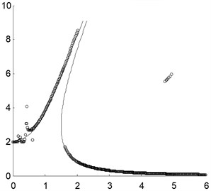
An illustrative example system is studied herein as defined by the basic system parameters $ω_{0} = 1$ , $ε = 0.05$ , $c = 0.2$ , $α = 1.3$ , $F = 1.5$ . Fig. 1 illustrates a comparison of the peak values of the approximately analytical solution by the presented method and the numerical solution in the frequency range $ω \in [1, 6]$ . The values of the approximately analytical solution are denoted by the solid line, while the values of the numerical results are indicated by the circle. It could be found that the approximately analytical solution agrees very well with the numerical results in the given frequency range except two small regions. The first region is the frequency range for super-harmonic resonance around $ω = 1/3$ , where the presented method could not open out the jump and hysteresis phenomenon in this range. But the range is small, and the peak values in this range are not large compared with those of the whole amplitude-frequency curves. The second region is the frequency range for the sub-harmonic resonance larger than $ω = 3$ , where the presented method could not interpret the multi-value phenomenon of the amplitude, and the amplitude of the sub-harmonic resonance by the numerical integration is large. Nevertheless, the existing range for the sub-harmonic is small, so that one could omit it in many practical engineering.

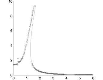
The effects of some important system parameters on the amplitude-frequency are also researched. For example, when the damping coefficient is selected as $c = 0.02$ and $c = 0.6$ , the results are shown in Fig. 2. It could be found that when the damping coefficient is smaller, the difference of the results between the approximately analytical solution and the numerical integration would be larger, and the sub-harmonic resonance would be more distinct. If the damping coefficient is larger, the sub-harmonic resonance would vanish and the two results would agree very well with each other, and the difference of the results between the approximately analytical solution and the numerical integration would be neglectable.

Fig. 1Comparison of the peak values of the approximately analytical solution by the presented method and the direct numerical integration for the basic system parameters: the solid line for the approximately analytical solution and the circles for the direct numerical integration

Comparison of the peak values of the approximately analytical solution by the presented method and the direct numerical integration for the basic system parameters: the solid line for the approximately analytical solution and the circles for the direct numerical integration

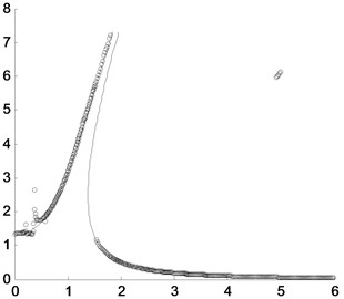
Fig. 2Comparison of the peak values of the approximately analytical solution by the presented method and the direct numerical integration where the solid line is for the approximately analytical solution and the circles are for the direct numerical integration with different damping coefficients: a) c=0.02; b) c=0.6

Comparison of the peak values of the approximately analytical solution by the presented method and the direct numerical integration where the solid line is for the approximately analytical solution and the circles are for the direct numerical integration with different damping coefficients: a) c=0.02; b) c=0.6

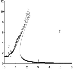
a)

b)

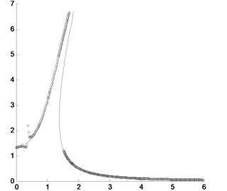
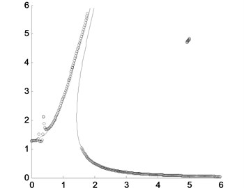
Fig. 3Comparison of the peak values of the approximately analytical solution by the presented method and the direct numerical integration where the solid line is for the approximately analytical solution and the circles are for the direct numerical integration with different amplitudes of excitation force: a) F=0.5; b) F=2.5

a)

b)

When the amplitude of excitation force is changed, for example, $F = 0.5$ and $F = 2.5$ , the amplitude-frequency curves obtained by the presented method and the numerical integration are shown in Fig. 3. It could be found that when the amplitude of excitation force is small enough, the sub-harmonic resonance disappears and the super-harmonic resonance is so small as to be neglectable. If the amplitude of excitation force is large enough, the sub-harmonic and super-harmonic resonance would all be obvious. But the amplitude of super-harmonic resonance and the existing range of sub-harmonic resonance are all small.

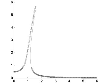
If the nonlinear stiffness coefficient is changed, for example, $α = 0.5$ and $α = 2.1$ , the amplitude-frequency curves obtained by the presented method and the numerical integration are shown in Fig. 4. It could be found that when the nonlinear stiffness coefficient is small, the sub-harmonic resonance would disappear and the super-harmonic resonance is very small. If the nonlinear stiffness coefficient is large enough, the sub-harmonic and super-harmonic resonance would all be clear. But the amplitude of super-harmonic resonance and the existing range of sub-harmonic resonance are still small.

Fig. 4Comparison of the peak values of the approximately analytical solution by the presented method and the direct numerical integration where the solid line is for the approximately analytical solution and the circles are for the direct numerical integration with different nonlinear stiffness coefficients: a) α=0.5; b) α=2.1

a)

b)

Comparatively speaking, the amplitude-frequency curves obtained by the presented method agree well with the numerical integration, which could make us research the nonlinear problems more convenient.

6. Conclusions

In this paper a revised averaging method is presented, which is entirely equal to the results of the primary resonance of the traditional averaging method. It is unnecessary to introduce the small dimensionless parameter and the detuning factor, which makes the solving procedure more convenient. Moreover, the general forms of the approximate solution of nonlinear system with only polynomial-type displacement nonlinearity are obtained. The Duffing oscillator, as an example, is researched and the results show the validity of the presented method.

References

Krylov N. N., Bogoliubov N. N. Introduction to Nonlinear Mechanics. Princeton University, Princeton, 1947.

Search CrossRef
Bogoliubov N. N., Mitropolskii Y. A. Asymptotic Methods in the Theory of Nonlinear Oscillations. Gordon and Breach, New York, 1961.

Search CrossRef
Sanders J. A., Verhulst F., Murdock J. Averaging Methods in Nonlinear Dynamical Systems. 2nd ed., Springer Science Business Media, New York, 2007.

Search CrossRef
Burd V. Method of Averaging for Differential Equations on an Infinite Interval: Theory and Applications. Taylor & Francis Group, 2007

Search CrossRef
Wang Z. H., Hu H. Y., Wang H. L. Robust stabilization to non-linear delayed systems via delayed state feedback: the averaging method. Journal of Sound and Vibration, Vol. 279, Issue 3-5, 2005, p. 937-953.

Search CrossRef
Roy R. V. Averaging method for strongly nonlinear oscillators with periodic excitations. International Journal of Non-Linear Mechanics, Vol. 29, Issue 5, 1994, p. 737-753.

Search CrossRef
Chatterjee A. Harmonic balance based averaging: approximate realizations of an asymptotic technique. Nonlinear Dynamics, Vol. 32, Issue 4, 2003, p. 323-343.

Search CrossRef
Kumar D., Datta T. K. Response of nonlinear systems in probability domain using stochastic averaging. Journal of Sound and Vibration, Vol. 302, Issue 1-2, 2007, p. 152-166.

Search CrossRef
Ji J. C., Hansen C. H. Analytical approximation of the primary resonance response of a periodically excited piecewise nonlinear-linear oscillator. Journal of Sound and Vibration, Vol. 278, Issue 1-2, 2004, p. 327-342.

Search CrossRef
Ji J. C., Hansen C. H. On the approximate solution of a piecewise nonlinear oscillator under super-harmonic resonance. Journal of Sound and Vibration, Vol. 283, Issue 1-2, 2005, p. 467-474.

Search CrossRef
Yang X. D., Tang Y. Q., Chen L. Q., Lim C. W. Dynamic stability of axially accelerating Timoshenko beam: averaging method. European Journal of Mechanics A/Solid, Vol. 29, Issue 1, 2010, p. 81-90.

Search CrossRef
Li X. Y., Ji J. C., Hansen C. H. Dynamics of two delay coupled van der Pol oscillators. Mechanics Research Communications, Vol. 33, Issue 5, 2006, p. 614-627.

Search CrossRef
Yang S. P., Chen Y. S. The bifurcations and singularities of the parametrical vibration in a system with Davidenkov's hysteretic nonlinearity. Mechanics Research Communications, Vol. 19, Issue 4, 1992, p. 267-272.

Search CrossRef
Nayfeh A. H., Mook D. T. Nonlinear Oscillations. John Wiley & Sons, INC, 1979

Search CrossRef
Fidlin A. Nonlinear Oscillations in Mechanical Engineering. Springer-Verlag, Berlin, Heidelberg, 2006.

Search CrossRef
Polyanin A. D., Manzhirov A. V. Handbook of Mathematics for Engineers and Scientists. Taylor & Francis Group, LLC, 2007.

Search CrossRef
Bronshtein I. N., Semendyayev K. A., Musiol G., Muehlig H. Handbook of Mathematics. 5th ed., Springer-Verlag, Berlin, Heidelberg, 2007.

Search CrossRef

About this article

Received

21 March 2014

Accepted

26 May 2014

Published

30 June 2014

Keywords

averaging method

nonlinear oscillator

approximate solution

polynomial-type displacement nonlinearity

Acknowledgements

The authors are grateful to the support by National Natural Science Foundation of China (No. 11072158 and 11372198), the Program for New Century Excellent Talents in University (NCET-11-0936), and the Cultivation Plan for Innovation Team and Leading Talent in Colleges and Universities of Hebei Province (LJRC018).

This is an open access article distributed under the Creative Commons Attribution License, which permits unrestricted use, distribution, and reproduction in any medium, provided the original work is properly cited.