Implementation of swarm algorithm in modeling a flexible beam structure

1. Introduction

Process modeling is a technique of achieving mathematical model which describes the behavior of a dynamic system. System Identification is one of the modeling methods used to build the mathematical model using experimental data input and output. System Identification has been developed for many years and different views on the definition of System Identification have been established.

In [1], an equivalent model can be determined from a set of data input and output which is the basic of identification from a group of models for the system under test. In addition, in [2], the identification problem can be summed up as a type of mathematical expression which represents the essential characteristics of an objective system by a model. By understanding the objective system, a useful form of the system can be expressed by using the obtained model. Furthermore, [3] mentioned that three important elements in System Identification are the data, models and standards. It stated that the identification is the process of selecting a model which fits the original data in accordance with a criterion. On top of that, System Identification has been widely applied in linear and nonlinear system [5, 6] in different application such as automotive air conditioning [7], flexible plate structure [8], flexible manipulator system [9], and flexible appendage on satellite for autonomous control [10].

System Identification has also been implemented with intelligent application technique to search the unknown parameters in modeling. Particle Swarm Optimization (PSO) is an intelligent swarm optimization method regarding the behavior of system in food searching which is proposed by Kennedy and Eberhart in 1995 [22]. PSO technique has been widely applied by researchers to model a system in recent years. The unknown parameters in mathematical model can be obtained effectively and efficiently via PSO technique. In [11], a power system measurement based load is applied with PSO technique to develop a mathematical model of the system. Meanwhile, [12] had implement PSO to IIR adaptive System Identification problem. The PSO technique has been modified and improved which produces a better result compared to the RGA and basic PSO model.

The implementation of PSO in mechanical system for System Identification can be seen in [7], [8] and [9]. Hanim Yatim et al. had model the flexible manipulator system using PSO and RLS [9]. In [9], it showed that PSO has the advantages over RLS in parametric modeling of flexible manipulator system. In addition, Muhammad Sukri Hadi et al. implemented PSO technique to obtain the model of flexible plate structure system with Free-Free-Clamped-Clamped Edge [8]. The PSO model is compared with RLS model and found that PSO model has performed better than RLS model in terms of mean-square-error (MSE), one-step-ahead prediction (OSA) and correlation test within 95 % confidence interval. Furthermore, PSO technique has been applied in modeling of automotive air conditioning system by Md Lazin et al. [7]. An ARX model is developed using PSO and RLS which both models were validated using OSA, MSE and correlation test. The result showed that PSO technique has produce the best ARX model with the lowest MSE value compared to RLS method.

Meanwhile, Artificial Bee Colony (ABC) algorithm is also known as intelligent optimization technique that has been employed in process modeling by several researchers. The concept of ABC is based on the bees’ activities in nectar foraging. The advantages of ABC algorithm are easy to implement, broad applicability in complex function, robust, able to explore local solutions and global optimizer [16]. ABC algorithm has been studied and enhanced since its proposal introduced by Karaboga in 2005 [17]. The research based on ABC algorithm had been carried out in solving the nonlinear equation [18] and identification of linear system [19] such as linearized power system stabilization [20].

In this paper, a cantilever flexible beam structure is the system that will be manipulated as shown in Fig. 1. The beam structure is one of the types of flexible structures that has been popularly applied in various fields of mechanical engineering, for instance, submarine, airplanes, ships, etc. However, the flexible structure is always influenced by unwanted vibration easily which may lead to drawbacks such as fatigue, instability, structure damage and performance reduction. Therefore, the unwanted vibration must be reduced and controller by an intelligent controller. To achieve the best controller performance, the development of an appropriate and accurate model to represent the beam system is utmost important.

To develop the model of the beam system, Mohammad et al. had successfully implement PSO technique with dynamic spread factor inertia weight in modeling the flexible system [15]. Result showed that PSO technique has the capability to obtain the model of the beam system with a low MSE value and good correlation test. However, the ABC algorithm is still a very new method to model the flexible beam system. Hence, this paper applied PSO and ABC algorithm to obtain the mathematical model of the beam system via System Identification using data acquisition from a well-developed experiment test rig. Both models are compared and validated using MSE, OSA and correlation test within 95 % confidence interval.

In this paper, the introduction and literature review of this work is presented in Section 1. In Section 2, the description of System Identification is discussed in detail. Moreover, the description of PSO and ABC are both presented in Section 3 and Section 4 respectively. In addition, the description of methodology of the work is discussed in Section 5. Meanwhile, in Section 6, the simulation results and discussion for PSO and ABC are compared and presented. Lastly, the conclusion for this work is presented in Section 7.

Fig. 1The cantilever beam system

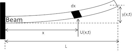
Fig. 2Concept of a simple black-box model with SISO

2. System identification

The modeling of a dynamic system is an important process to describe the characteristic and behavior of a system in term of mathematical equation. To achieve the best controller performance in control system, an appropriate model is required to be developed.

Two types of approaches to obtain the model of a dynamic system are discussed in [4]. It stated that one of the approaches for modeling a system is to create a fundamental model based on knowledge (physics and chemistry) of the system to be modeled. Such model is described as the ‘right’ model that provides the correct and actual behavior of the system. In addition, it is robust that can be applied repeatedly under any different conditions. However, it is the most difficult and time consumed way in obtaining all of the knowledge regarding the physical and chemistry of the system, especially if the system is complicated.

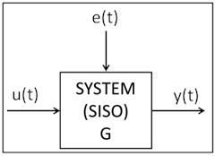
The second approach for modeling a system is using System Identification by choosing an appropriate mathematical form (or known as transfer function) that represents the behavior of the system via experimental data acquisition. This type of model is known as ‘black box’ or ‘input-output’ model which is convenient, simple and easy to manipulate. This model seeks to reproduce the behavior of the system’s output if only the set point or input has been changed. The advantage is the model can be developed without prior knowledge about the system; hence, the complicated system can be modeled easily and quickly.

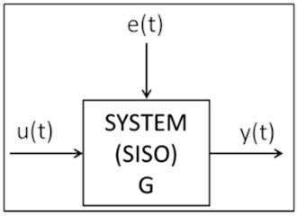
A simple black-box or input-output model is represented in Fig. 2. $u$ and $y$ are both denoted as the input and output of the system respectively. The output system will be changed in response of the change of inputs and time. Assume that $G$ is the plant system, the general transfer function in frequency domain is denoted as $G\left(s\right)=Y\left(s\right)/U\left(s\right)$. In control system, the controller performance depends on the identified plant model, $G\left(s\right)$ by using System Identification.

The system identification procedures are as following:

1) Experimental design and setup.

An analytical model of the structure is built and well-developed. All the instrumentation requirements needed are determined to collect the data input and output with prescribed accuracy and spatial resolution.

2) Perform the experiment.

The data input and output are collected from the experiment. The System Identification technique is implemented to the experiment data to obtain the mathematical model of the system.

3) Choosing a suitable model.

The model can be chosen using prior knowledge or trial-and-error. There are various types of model that can be considered as the model in System Identification, for instance, AR, ARX, ARMA, NARX, NARMA, etc.

4) Evaluate and validate the model.

The predicted model can be evaluated and validated by comparing the predicted output with the original output which is called as error. Correlation test can be brought out to test the relationship between the error and input. The best fit model always been selected if only the error is minimum and unbiased correlation test.

3. Particle swarm optimization

In 1995, Kennedy and Eberhart proposed Particle Swarm Optimization (PSO) algorithm which is a stochastic global optimization algorithm regarding the behaviors of the swarms such as flock of birds, schools of fish or swarm of bees in food searching. PSO has been widely used in various fields and application especially in modeling and control.

PSO involves the problem that needs to be solved which the fitness function, $f\left(x\right)$ is defined and to be minimized or maximized. A set of particles search their food in a search space repeatedly until the stopping criteria is met. Swarm is the set of potential solutions to the optimization problem where particle is the potential solution in the swarm set. The best solution achieved by the particle and swarm in a neighborhood are called as personal best position (denoted as $pbest$ in Eq. (1)) and global best position (denoted as $gbest$ in Eq. (2)) respectively. The $pbest$ and $gbest$ values found are always being memorized until the end of the searching. The previous memorized solution will be replaced and updated if there is a better solution compared to the previous solution:

where $x_{id}$ is the current position of the particle.

In PSO algorithm, each particle will be first initialized for its position and velocity randomly in a swarm set. It holds the position as the candidate solution to the problem and the velocity as the flying direction of the particle. The velocity and position will be updated using Eqs. (3) and (4) respectively in each iteration of solution searching process:

where $c_1$, $c_2$ are the acceleration constants, $r_1$ and $r_2$ are the random numbers with the value between 0 and 1. In [11], $c_1$ and $c_2$ are adjustable experimentally between 1 and 2. For a better control exploitation and exploration, the inertia weight is introduced as in Eq. (5):

Inertia weight $w$ serves as the memory of the previous direction to prevent the particle from changing direction drastically [9]. It can be updated using Eq. (6) to avoid $w$ from exceeding the number of iterations:

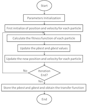
A basic procedure for PSO technique is presented in the flow chart as shown in Fig. 3.

4. Artificial bee colony

Artificial Bee Colony (ABC) algorithm involves the behavior of a bee in food foraging. ABC algorithm was proposed by Devis Karaboga in 2005 [17]. It was formed by observing the activities and behaviors of the real bees which were looking for the nectar resources and sharing the amount of nectar resources with the other bees.

In ABC algorithm, there are three essential components which are food sources, employed foragers and unemployed foragers. The food sources represent the solutions to the optimization problems. A forager bee identifies the quality of a food source, such as the taste of its nectar, nearness to the hive, and efficiency of the energy in order to choose a food source [21]. An employed forager acts as an information carrier of a specific food source and shares the information to other bees waiting in the hive. The information contains the distance between the hive and the food source, the direction and the cost of the food source [19]. An unemployed forager who may be an onlooker bee or scout bee looks for a food source to exploit. An onlooker bee attempts to search a food source regarding to the information shared by employed bee. A scout bee searches for a food source randomly without any knowledge and fact.

Fig. 3The flow chart of PSO algorithm

The steps in ABC algorithm are stated below:

1) Initialization population;

2) Repeat;

3) Place the employed bees on the food source;

4) Evaluate the food source and share to onlooker bees;

5) Place the onlooker bees on the discovered food source based on the information shared by employed bees;

6) Evaluate the food source;

7) Send a scout bee for searching new food source;

8) Memorize the best food source found so far;

9) Until requirements are met.

In the first initialization, a set of food source with a particular range of the variables $x_i$ ($i=$ 1, 2,…, $SN$) is randomly selected by the bees. The initial amount of nectar source is determined and the best food source is memorized.

In ABC algorithm, half of the bees in colony are chosen as employed bees and another half for onlooker bees. In the first step of ABC, the employed bees will search a new set of food source using Eq. (7) and evaluate the food via a fitness function in Eq. (8). The information of the food source will be memorized and shared to the onlooker bees waiting in the hive. The onlooker bees observe, evaluate and choose the food source via the dances presented by employed bees:

where $k\in (i=\text{1, 2,…,}SN)$, $j\in \left\{\text{1,2,…,}D\right\}.$$k$ is generated by $int\left(rand,SN\right)+1$ while $SN$ is the number of food source. $j$ is one-dimensional variable in $D$ dimensional vector. Both $k$ and $j$ are randomly generated with $k\ne i$. ${\varphi }_{ij}$ is a random number between –1 and 1.

The fitness function for the food evaluation after the discovery of the source is denoted as in Eq. (8):

where $f_i$ is the cost function of solution $i$.

In the second step of ABC, onlooker bees make a resource choice depending on the probability value in Eq. (9) associated with the food source:

where $fi{t}_i$ – fitness value of solution $i$.

The onlooker bees will search for new solutions within the resource chosen using Eq. (7) and evaluate the food via fitness function in Eq. (8). The greedy selection process is applied if there is a better food source compared to the previous one. The previous food source will be replaced by the new better food source.

In the third step, a scout bee has been selected from the abandoned employed bee. If the abandoned source is unable to be improved anymore, the abandoned employed bee will become as a scout bee to identify a new resource in the search space without any prior knowledge and fact.

Assume that the abandoned source is $x_i$ with $j\in \{\mathrm{1,2},\dots ,D\}$, then the scout discovers a new food source to replace the previous $x_i$ based on Eq. (10):

5. Methodology

5.1. Experiment setup

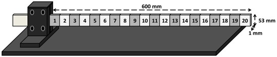
In this paper, a cantilever beam is selected as flexible beam structure as shown in Fig. 4. The cantilever beam is made of aluminum with the length 600 mm, thickness 1mm and width 53 mm. The parameters regarding the physical measurement of cantilever beam are listed in Table 1. The beam has been equally divided into 20 segments as shown in Fig. 5. The divided segment is used to determine the actuators’ and sensors’ location. In this paper, disturbance actuator, control actuator, detection sensor and observation sensor are placed at the segments between 8th and 9th, 10h and 11th, 9th and 10th, 19th and 20th respectively as shown in the schematic diagram Fig. 6. The base is built to ensure the beam structure is clamped strongly and stable in order to prevent any immeasurable noise to disturb the beam system.

The beam system applied in this paper is presented in the schematic diagram Fig. 6. This system requires several important components which are piezoelectric patches, amplifiers, DAQ connector block, DAQ card, personal computer (PC) and software platform using MATLAB SIMULINK. These required components with each specification are listed in Table 2. In this system, four piezoelectric patches with the same types of PI P-876.A11 are required as the sensors and actuators which are mounted on both sides of the beam structure. The disturbance actuator is used to vibrate the beam while the control actuator is used to control and reduce the vibration of the beam based on the controller output given. In addition, the detection sensor is used to detect the input that beam experienced while the observation sensor is used to observe the motion and vibration of the beam structure at a certain point of the beam structure. However, in this paper, the control actuator is mounted at the beam for modeling purpose only.

Fig. 4The cantilever beam system

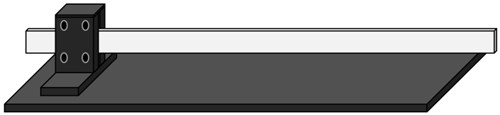
Fig. 5Physical measurement of cantilever beam with 20 segments division

Apart from that, another important component in this system is amplifier. The signals generated from PC and piezoelectric sensors are amplified by amplifiers in voltage. Furthermore, a DAQ connector block is used as a signal conditioning block which consists of ADC and DAC. The block is connected to the DAQ card and amplifiers. The DAQ card is installed in the PC with port PCI. On top of that, another important component used in this system is the software platform. In this paper, the MATLAB SIMULINK blocks are developed to collect the data input and output from experiment for modeling purpose.

There are four piezoelectric patches mounted at the sides of beam structure as shown in the schematic diagram Fig. 6. Each piezoelectric patch requires an amplifier for signal amplification. This system starts with the generation of disturbance signal from the PC. The signal is sent to actuator after digital-analog conversion in DAQ system. In this paper, a sinusoidal signal is selected as the disturbance to the beam system. The signal is transmitted in voltage from DAQ connector block to the amplifier E-835 and then to the piezoelectric actuator. The piezoelectric patch will start bending after receiving the voltage signal at the disturbance point on the beam and thus to vibrate the beam. Meanwhile, the piezoelectric sensors will sense the vibration at the detection and observation points. The signals sensed are transmitted to the DAQ system in order to allow the computer understands and read the signal retrieved after the amplification using amplifiers E-413. The signals can be displayed in MATLAB SIMULINK scope to allow the user observes the vibration and stores the data input and output for System Identification purpose.

Table 1Specification of cantilever beam structure

Beam structure	Specification
Material	Aluminum
Length	600 mm
Width	53 mm
Thickness	1 mm

Table 2Tools requirement with specification and functionality

Tools	Quantity	Specification	Functionality
Piezoelectric patches	4	PI P-876.A11	Sensor and actuator
Amplifiers (1)	2	E-835 DuraAct	Amplification
Amplifiers (2)	2	E-413 DuraAct	Amplification
DAQ Card	1	NI-DAQ PCI-6259	Data acquisition
DAQ connector block	1	SCC-68 M Series	Signal conditioning
Personal computer	1	HP Intel I7-3770	Computation
Beam	1	Aluminum	Flexible structure
Software	1	MATLAB R2012A	Graphical user interface

In this paper, data acquisition is simulated using MATLAB SIMULINK Toolbox which is installed in the PC and integrated to the experimental test rig. The data acquisition system for obtaining the data input and output is shown in Fig. 7. The main components of data acquisition system are analog input, analog output, low pass filter and disturbance source. The analog input is connected to the sensors where the signals of vibration are retrieved. Apart from that, the analog output is connected to disturbance and control actuators that used to vibrate and control the beam structure respectively.

Fig. 6Schematic diagram of the cantilever beam system

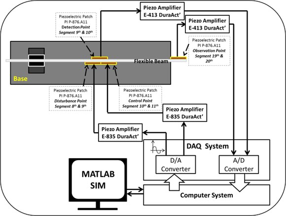
Fig. 7The block diagram of data acquisition system using Matlab Simulink toolbox

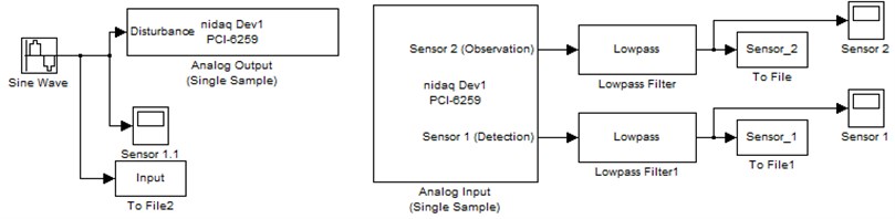
Fig. 8The settings of analog input

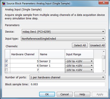
Fig. 9The settings of analog output

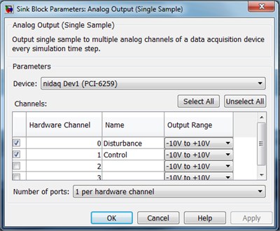
The PCI-6259 National Instrument DAQ card is used for data acquisition system. The settings of the analog input and output are shown in Fig. 8 and Fig. 9 respectively. The device for analog input and output is nidaq Dev1 (PCI-6259) with the hardware channel AI6 and AI5, and AO0 respectively. The input type for analog input is set as “Non Referenced Single Ended” (NRSE) with the input range of –10V to +10V and 0.003 sampling time. The low pass filter is used to eliminate the noise caused by the wiring connection and electrical components in the system.

In this paper, a 4 V sine wave with frequency 2 Hz is generated as the force disturbance to the beam system as shown in Fig. 10. The disturbance signal is sent via the analog output to the actuator.

The motion of the beam that sensed from piezoelectric sensors can be observed from the scopes of sensor 1 and sensor 2 in the block diagram Fig. 7. The data input and output are saved in mat file for System Identification purpose.

Fig. 10The settings of sine wave disturbance

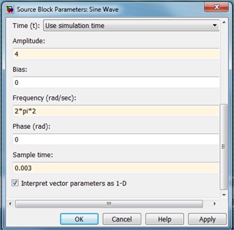
Fig. 11The SISO system G

5.3. Particle swarm optimization

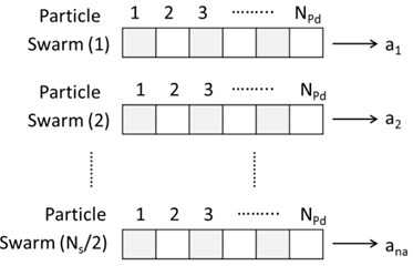
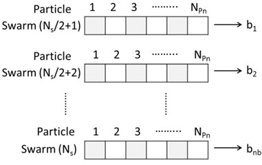
Particle Swarm Optimization algorithm is simulated using MATLAB environment in this paper. Next, the numbers of swarm sets are determined based on the number of estimated parameters, $N_s=OrderNumber\times 2$.

Each swarm set represents one estimated parameter for numerator or denominator. The numbers of swarm sets of estimated parameters for numerator and denominator are the same: $(na=nb=N_s/2)$.

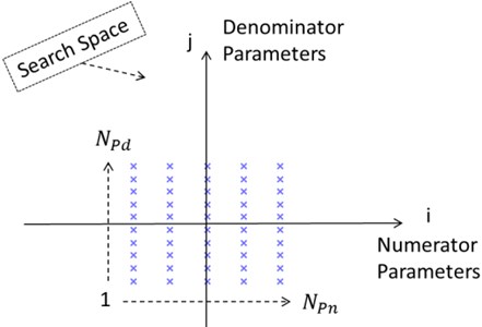
For instance, assume that the algorithm consists of 10 swarm sets; 5 sets of the swarm are used to estimate the denominator parameters and another 5 sets for numerator parameters. Each particle holds the information of position in the search space. The number of particle for numerator $N_{Pn}$ and denominator $N_{Pd}$ are determined by 2 dimensional $i\times j$ of a swarm set as in Fig. 12.

Estimated parameters vector:

19

$\mathrm{\theta }=\left[\begin{array}{l}{a}_1\\ ⋮\\ a_{na}\\ b_1\\ ⋮\\ b_{nb}\end{array}\right]\to \left[\begin{array}{l}{j}_1\\ ⋮\\ j_{N_{Pd}}\\ i_1\\ ⋮\\ i_{N_{Pn}}\end{array}\right].$

In the first initialization, each particle is given a random position around the origin (0, 0) as in Fig. 13 and solves the fitness function for the first time to obtain the first best particle (“pbest”) and global (“gbest”) position. After that, each particle in every swarm set will find a new position in the following iteration based on the new velocity obtained from Eq. (3). The new position for each particle will be used to solve the fitness function again. The values of “pbest” and “gbest” will be updated based on the best value obtained from fitness function. In the end of iteration, all the particles in each swarm sets will gather at the same position which is the best optimal solution to the fitness function.

Fig. 12The structure of the swarms in PSO

a) Denominator

b) Numerator

Fig. 13First initialization of swarms’ position

5.4. Artificial bee colony

Artificial Bee Colony algorithm is simulated in MATLAB environment to obtain the mathematical model of a flexible beam structure. The experimental data input and output are collected and imported into MATLAB. The parameters required to be determined in ABC algorithm are listed in Table 3.

Table 3The parameters required in ABC algorithm

No.	Parameters	No.	Parameters
1.	Size of colony	6.	Range of search space, $L$
2.	Number of food source	7.	Limit trial number
3.	Maximum cycle	8.	Number of employed bees
4.	Sampling time	9.	Number of onlooker bees
5.	Model order number

The algorithm starts with the initialization of the food source. The food source is set initially random in the particular range of search space. The initial food source will be evaluated and determined via the cost function and fitness function. The mean-square-error (MSE) of the error between predicted data and experimental data will be the cost function for ABC algorithm in this paper. The best food source found will be stored in the memory.

ABC algorithm consists of two phases which are employed bee phase and onlooker bee phase. In the employed bee phase, each employed bee holds the solutions for the values of numerator ($a_1$, $a_2$,…, $a_{na}$) and denominator ($b_1$, $b_2$,…, $b_{nb}$) as indicated in Fig. 14(a).

Each employed bee will update its food source randomly using Eq. (7) and evaluate it via fitness function in Eq. (8). If the random food source from Eq. (7) is exceeding the particular range of search space, it will be randomly picked repeatedly until it is obtained in the desired range. If there is a better fitness value obtained compared to the previous, that particular food source will be updated and stored. The information of food source will be shared with the onlooker bees.

In onlooker bee phase, the onlooker bees will select the food source regarding to the probability in Eq. (9). Each onlooker bee has the solutions for the values of numerator ($a_1$, $a_2$,…, $a_{na}$) and denominator ($b_1$, $b_2$,…, $b_{nb}$) as in Fig. 14(b).

Each onlooker bee will update its food source randomly using Eq. (7) and evaluate it via fitness function in Eq. (8). If the random food source from Eq. (7) is exceeding the particular range of search space, it will be randomly picked repeatedly until it is obtained in the desired range. If there is a better fitness value obtained compared to the previous, that particular food source will be updated and stored. In this paper, if the food source consists of a better solution compared to the previous, it will be stored in the memory known as “GlobalParams”.

Fig. 14The structure of employed bee and onlooker bees

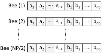
a) Employed bee

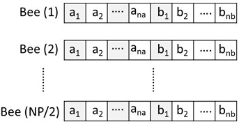
b) Onlooker bees

However, if there is a food source that has been abandoned exceeds the limit trial numbers, the employed bee which holds that abandoned food source will become a scout bee. It will search a new random food source using Eq. (10) without any knowledge and fact. The fitness of food found will be evaluated using Eq. (8). If there is a better fitness value compared with the previous one, the abandoned food source will be stored in the memory.

6. Results and analysis

6.2. Particle swarm optimization

In PSO technique, all the parameters required are set as in the Table 4. The PSO algorithm is simulated using MATLAB coding which produces the results in graphical plots and numerical values. The system is simulated from 2nd to 10th order number and comparison of validation result for each order number is showed in the Table 5.

Fig. 15The disturbance input with sinusoidal signal

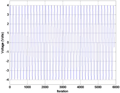
Fig. 16a) The disturbance sensed at detection point on the beam, b) the vibration of the beam at 19th and 20th segments

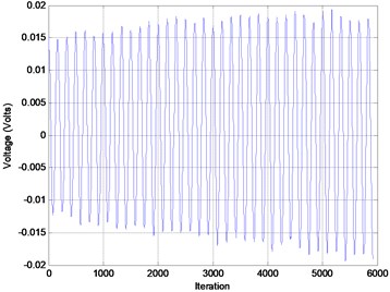
a) Detection of the input disturbance

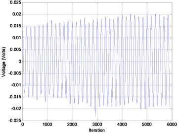
b) Obdervation of the output vibration

From the results obtained in Table 5, it can be observed that an 8th order model yields good result in term of correlation tests which are within 95 % confidence interval. However, a 3rd order model is considered as the best fit model of the flexible beam system in this work. This is because it yields a stable model with the lowest MSE value with 1.9016×10^-10 although its correlation tests are slightly exceeding 95 % interval confidence.

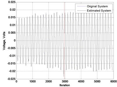
In addition, the comparison of estimated data and original data of beam system in time domain is plotted in Fig. 17. The result shows that a 3rd order system can yield a predicted output that almost similar to the real output of the beam system.

The vibration modes for predicted model and original data output are compared and plotted in Fig. 18. Result shows that the 3rd order predicted model has the same natural frequencies with the original system in the first 2 vibration modes.

Table 4The parameters required in PSO algorithm

Parameters	Values
Sampling time, $dt$	0.003
Correction factor, $b_1=b_2$	2.0
Number of iteration	1500
Size particle	20×30
Range of inertia	0.15-0.95

Table 5The comparison of MSE values and correlation test with different order number for PSO model

Order	MSE	ACR	CCR
2	1.3970×10-9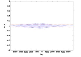
3	1.9016×10-10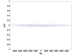
4	1.6879×10-9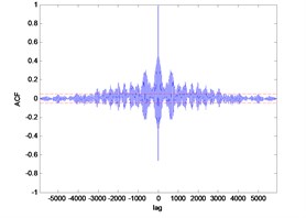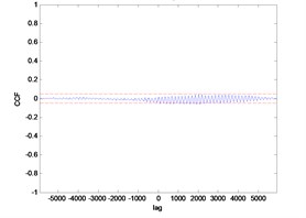
5	4.5122×10-9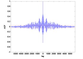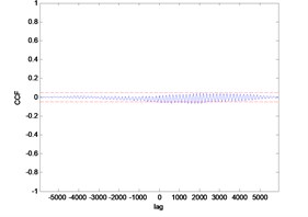
6	1.4880×10-9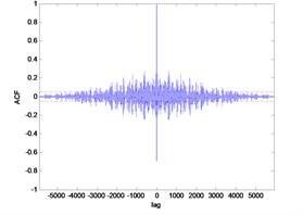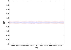
7	2.2448×10-9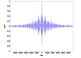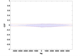
8	6.1953×10-9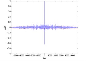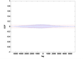
9	3.4093×10-9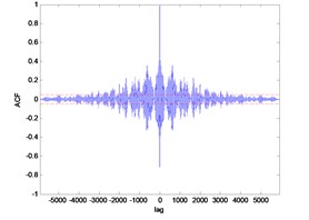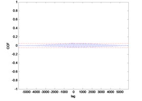
10	3.5040×10-9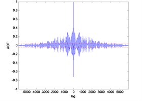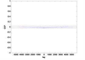

The ARX model $G_{PSO}$ with 3rd order system in zero order hold is presented in Eq. (20). The 3rd order model can be selected for controller design with the PSO application as the model is stable and closed to the real beam system:

20

$G_{PSO}=\frac{0.2489z^{-1}-0.4296z^{-2}+0.1835z^{-3}}{1-2.415z^{-1}+1.907z^{-2}-0.4901z^{-3}}.$

Fig. 17The vibration of the beam in time domain modeled by PSO algorithm

6.3. Artificial bee colony

In ABC technique, all the parameters required are set as in the Table 6. The ABC algorithm is simulated using MATLAB coding which produces the results in graphical plots and numerical values. The system is simulated from 2nd to 10th order number and comparison of validation result for each order number is showed in the Table 7.

From the results obtained in Table 7, it can be observed that a 10th order model yields good result in term of correlation tests which are within 95 % confidence interval. However, a 2nd order model is considered as the best fit model of the flexible beam system in this work as it yields a stable model with the lowest MSE value with 2.1723×10^-9 although its correlation tests are exceeding 95 % interval confidence.

Fig. 18The comparison of vibration modes between the predicted model and the real system

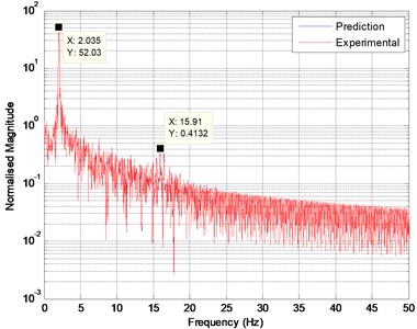
Table 6The parameters required in ABC algorithm

Parameters	Values
Sampling time, $dt$	0.003
Number of population	300
Maximum cycle	1500
Number of employed bees	150
Number of onlooker bees	150
Limit of trial number	15
Range for searching area	[rand*2.5]+0.5

In addition, the comparison of estimated data and original data of beam system in time domain is plotted in Fig. 19. The result shows that a 2nd order system can yield a predicted output that almost similar to the real output of the beam system.

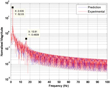
The vibration modes for predicted model and original data output are compared and plotted in Fig. 20. Result shows that the 2nd order predicted model has the same natural frequencies with the original system in the first 2 vibration modes.

The ARX model $G_{ABC}$ with 2nd order system in zero order hold is presented in Eq. (21):

21

$G_{ABC}=\frac{0.347z^{-1}-0.3432z^{-2}}{1-1.673z^{-1}+0.6763z^{-2}}.$

From the results obtained using PSO and ABC, it can be seen that both of the models have the same natural frequencies for the first 2 vibration modes. In addition, both models consist of a very low MSE value with low order number. Furthermore, both of the 3rd order PSO model and 2nd order ABC model produce stable system. However, in terms of MSE value and correlation tests, the 3rd order PSO model yields the lowest MSE value of 1.9016×10^-10 and correlation tests within 95 % confidence interval. Meanwhile, the correlation tests of 2nd order ABC model show that the behavior of the model has less significant correlation between the input and residual compared to 3rd order PSO model. Hence, the 3rd order PSO model is considered as the most suitable model to represent the beam system in this paper.

Table 7The comparison of MSE values and correlation test with different order number for ABC model

Order	MSE	ACR	CCR
2	2.1723×10-9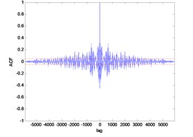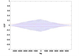
3	1.2375×10-8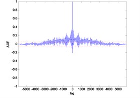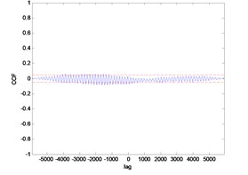
4	6.3966×10-9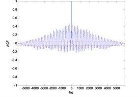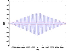
5	1.9368×10-8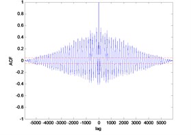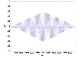
6	2.0471×10-8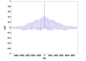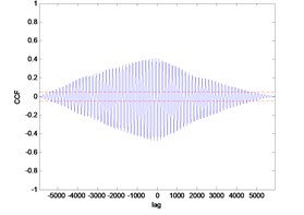
7	2.9549×10-8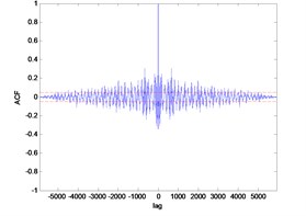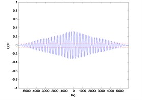
8	4.6066×10-8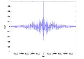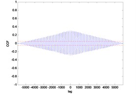
9	4.7791×10-8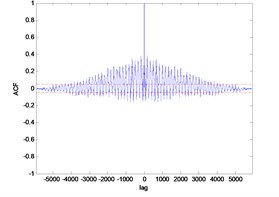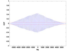
10	4.6055×10-8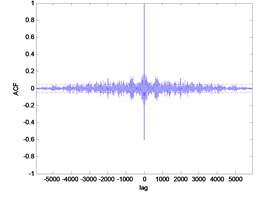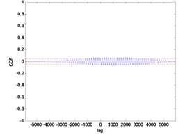

Fig. 19The vibration of beam in time domain modeled by ABC algorithm

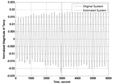
Fig. 20The comparison of vibration modes between the predicted model and the real system

7. Conclusion

This paper proposed the optimization techniques which are applied in System Identification for modeling a flexible beam system. An experiment test rig for the beam system is built and developed to collect the data input and output experimentally for System Identification. Furthermore, a linear ARX model is estimated to be the model of the beam system. The optimization techniques are applied to estimate the unknown parameters in the ARX model. On top of that, several validation tests such as MSE and correlation tests are carried out to ensure the predicted model is close to the real system. In this paper, Particle Swarm Optimization and Artificial Bee Colony are the techniques used for parameters estimation of an ARX model.

From the results obtained by PSO technique, a 3rd order model is selected as the best fit model with the lowest MSE value of 1.9016×10^-10. Its correlation tests show that the PSO model is within the 95 % confidence interval and close to the real system. Furthermore, in time domain, the predicted output is the same as the original output taken from experiment. Moreover, the natural frequencies for the first 2 vibration modes of the predicted model and original system are the same as well.

Meanwhile, it can be observed that ABC technique is able to develop a 2nd order model with a low MSE value of 2.1723×10^-9. In time domain, the predicted output is exactly the same as the original output taken from experiment. Apart from that, the natural frequencies for the first 2 vibration modes of the predicted model and original system are similar. However, based on the correlation tests, the behavior of ABC model is biased and less significant relationship between the input and residual compared to the 3rd order PSO model. Hence, the 2nd order ABC model is unable to represent the real system of the flexible beam structure. On the contrary, the PSO model is the most appropriate and suitable as the predicted model for the flexible beam system as it consists of the lowest MSE and good correlation tests between the input and residual.

In the future work, the PSO model obtained will be validated through the real experiment by designing a controller to suppress the vibration of the beam system. The vibration must be reduced using this PSO model with the controller such as PID, direct controller, etc. Furthermore, Artificial Bee Colony is still a very new intelligence algorithm. It can be modified and improved for modeling in order to obtain an appropriate and accurate model of the beam system.