Comparing PID and H-infinity controllers on a 2-DoF nonlinear quarter car suspension system

Papkollu, Kousik; Singru, Pravin M.; Manajrekar, Narayan

Journal of Vibroengineering

Browse Journal

Submit article

Published: 30 December 2014

Check for updates

Comparing PID and H-infinity controllers on a 2-DoF nonlinear quarter car suspension system

Kousik Papkollu¹

Pravin M. Singru²

Narayan Manajrekar³

^{1, 2}Department of Mechanical Engineering, BITS Pilani K. K. Birla Goa Campus, Goa, India

³nt of Electrical and Electronics Engineering, BITS Pilani K. K. Birla Goa Campus, Goa, India

Corresponding Author:

Kousik Papkollu

Cite the article Download PDF

Downloads 1558

Abstract

Automotive suspension system is an important part of car comfort and safety. In this article active suspension for 2DOF nonlinear coupled Passenger-Car model with force actuator is designed using PID control and H-infinity control. This paper is focused on comparison of those two controllers. Simulations on an exact nonlinear model of the suspension are performed for control validation.

1. Introduction

The fundamental task of suspension systems is to isolate the forces transmitted by external excitation. The problem of mechanical vibration control is generally tackled by placing suspension systems between the source of vibration and the structure to be protected. The suspension systems are composed of spring type elements in parallel with dissipative elements. They are employed in mobile applications, such as automobiles, or in non-mobile applications like vibratory machinary or civil structures. In the case of automobile, the suspension aims to achieve isolation from road by means of spring type elements and viscous dampers and contemporarily to improve road holding and handling [1, 2].

In general, a good suspension should provide a comfortable ride and good handling within a reasonable range of deflection. Moreover, these criteria subjectively depend on the purpose of the vehicle. Racing and sports cars generally have stiff suspensions with poor ride quality and good road handling while luxury cars have softer suspensions with good ride quality and poor road handling capabilities. Passive suspension design is traditionally done as compromise between spring and damper design. It is a tradeoff between ride comfort and vehicle handling/stability. These two criteria are conflicting. If damping is low, then ride comforts are good, but vehicle stability is low/poor and vice versa. So a compromise between these two conflicting criteria has to be obtained if suspension is to be developed by using passive spring and damper. In order to build a safer and more comfortable car out of passive component is hence difficult. This lead to the development of active suspension system. From a system design point of view, there are mainly two types of disturbances on a vehicle, namely road and load disturbances. Road disturbances have the characteristics of large magnitude in low frequency (such as speed breakers, bumps) and small magnitude in high frequency (such as road roughness). Load disturbances include the variation of loads induced by accelerating, braking and cornering. A suspension system needs to be soft against road disturbances and hard against load disturbances [2, 3].

1.1. Active suspension systems

The inherent limitations of classical suspensions have motivated the investigation of controlled Active suspension systems. Demands for better ride comfort and controllability of road vehicles has motivated many automotive industries to consider the use of active suspensions. These electronically controlled active suspension systems can potentially improve the ride comfort as well as the road handling of the vehicle simultaneously. An active suspension system should be able to provide different behavioral characteristics depending upon various road conditions, and be able to do so without going beyond its travel limits.

A vast amount of work on controlled suspension systems is present in technical and scientific literature. The first paper dealing with active suspensions dates back to 1950s [4]. Also, active vehicle suspensions have attracted a large number of researchers in the past few decades, and comprehensive surveys on related research are found [5-9]. Various approaches have been proposed to improve the performance of active suspension designs, such as linear optimal control [10], fuzzy logic and neural network control [11], adaptive control [12], H-infinity control [13], nonlinear control [14], gain-scheduling control [15] and preview control [16].

1.2. Biodynamics of seated human

Humans are most sensitive to whole body vibration under low-frequency excitation in seated posture. As a result, biodynamics of seated human subjects has been a topic of interest over the years. One of the early studies on the biomechanics of seated drivers subject to vibration was realized by Suggs et al., where the human body was modeled as a damped spring-mass system to build a standardized vehicle seat testing procedure [17]. Muksian and Nash [18] and Pope et al. [19] investigated the response of seated humans to sinusoidal vibration and impact. A detailed experimental work on translational seat vibration was performed by Griffin et al. to determine the effects of level, frequency and direction of the seat vibration [20]. Dynamic response of a seated subject was investigated in various aspects, for example, the effect of various cushions [21], the effect of vibration frequency and posture [22]; Wilder et al., [23], and the effect of backrest [24-25]. Wan and Schimmels [26] established a seated human body model to design an optimal seat suspension for isolation of the vertical WBV based on the simulated subjective response. On the other end of the spectrum, the effect of spinal forces due to WBV [27-29] and sitting biomechanics were considered in some other studies [30-33].

2. Non-linear coupled passenger car model

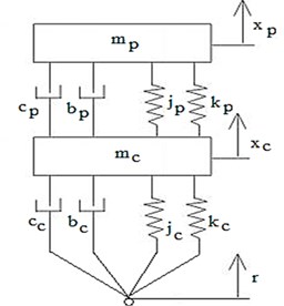
It is widely accepted that a quarter-car model is adequate for studying some vehicle suspension performance goals [34-35]. In this case, vehicle roll and pitch motion are ignored and the only degrees of freedom included are the vertical motion of the car and passenger. A typical quarter-car suspension system with MR damper is shown in Fig. 1. The subscript $p$ and $c$ denoted the passenger and car parameters respectively. $k_{p}$ and $k_{c}$ were linear stiffness coefficients whereas $j_{p}$ and $j_{c}$ were cubic stiffness coefficients. Likewise, $c_{p}$ and $c_{c}$ were linear damping coefficients. Further, $b_{p}$ and $b_{c}$ were cubic damping coefficients which is the inherent nonlinearity in the given system. To derive the equations of motion of this system, Lagrange’s energy method was used [36].

Fig. 1Non-linear coupled passenger car model

The equations of motion were obtained as:

1

m_{p} {\ddot{x}}_{p} + k_{p} (x_{p} - x_{c}) + j_{p} {(x_{p} - x_{c})}^{3} {+ c}_{p} ({\dot{x}}_{p} - {\dot{x}}_{c}) + b_{p} {({\dot{x}}_{p} - {\dot{x}}_{c})}^{3} = 0,

2

m_{c} {\ddot{x}}_{c} - k_{p} (x_{p} - x_{c}) - j_{p} {(x_{p} - x_{c})}^{3} - c_{p} ({\dot{x}}_{p} {- \dot{x}}_{c}) - b_{p} {({\dot{x}}_{p} - {\dot{x}}_{c})}^{3} + k_{c} (x_{c} - r)

+ j_{c} {(x_{c} - r)}^{3} + c_{c} ({\dot{x}}_{c} - \dot{r}) + b_{c} {({\dot{x}}_{c} - \dot{r})}^{3} = 0 .

The equations of motion derived in the previous section were nonlinear. To implement these equations in Simulink, it was essential to separate the state variables and to reduce Eqs. (1) and (2) into a convenient form for analysis. There were 4 state variables to this system. Letting $x_{1} = x_{p}$ , $x_{2} = {\dot{x}}_{p}$ , $x_{3} = x_{c}$ , $x_{4} = {\dot{x}}_{c}$ .

The equations of motion were rewritten as:

3

{\dot{x}}_{1} = x_{2},

4

{\dot{x}}_{2} = \frac{- 1}{m_{p}} (k_{p} (x_{1} - x_{3}) + j_{p} {(x_{1} - x_{3})}^{3} {+ c}_{p} (x_{2} - x_{4}) + b_{p} {(x_{2} - x_{4})}^{3}),

5

{\dot{x}}_{3} = x_{4},

6

{\dot{x}}_{4} = {\frac{1}{m_{c}} (k}_{p} (x_{1} - x_{3}) + j_{p} {(x_{1} - x_{3})}^{3} + c_{p} (x_{2} {- x}_{4}) + b_{p} {(x_{2} - x_{4})}^{3} - k_{c} (x_{3} - r)

- j_{c} {(x_{3} - r)}^{3} - c_{c} (x_{4} - \dot{r}) - b_{c} {(x_{4} - \dot{r})}^{3}) .

The following parameters were chosen for simulation [36]: $m_{p} =$ 60 kg, $m_{c} =$ 240 kg, $k_{p} =$ 25000 N/m, $k_{c} =$ 160000 N/m, $j_{p} =$ –2500 N/m³, $j_{c} =$ –300000 N/m³, $c_{p} =$ 200 Ns/m, $c_{c} =$ 250 Ns/m, $b_{p} =$ –10 Ns³/m³, $b_{c} =$ –25 Ns³/m³.

The fixed points of the system for Eqs. (3)-(6) are calculated as follows:

[\begin{matrix} {x_{1}}^{*} \\ {x_{2}}^{*} \\ {x_{3}}^{*} \\ {x_{4}}^{*} \end{matrix}] = \{[\begin{matrix} 0 \\ 0 \\ 0 \\ 0 \end{matrix}], [\begin{matrix} \pm \sqrt{\frac{- k_{p}}{j_{p}}} \\ 0 \\ 0 \\ 0 \end{matrix}], [\begin{matrix} \pm \sqrt{\frac{{- k}_{c}}{j_{c}}} \\ 0 \\ \pm \sqrt{\frac{{- k}_{c}}{j_{c}}} \\ 0 \end{matrix}], [\begin{matrix} \pm \sqrt{\frac{{- k}_{c}}{j_{c}}} \pm \sqrt{\frac{{- k}_{p}}{j_{p}}} \\ 0 \\ \pm \sqrt{\frac{{- k}_{c}}{j_{c}}} \\ 0 \end{matrix}]\} .

With above mentioned values of the parameters fixed points are found as given below:

[\begin{matrix} {x_{1}}^{*} \\ {x_{2}}^{*} \\ {x_{3}}^{*} \\ {x_{4}}^{*} \end{matrix}] = \{[\begin{matrix} 0 \\ 0 \\ 0 \\ 0 \end{matrix}], [\begin{matrix} \pm \sqrt{10} \\ 0 \\ 0 \\ 0 \end{matrix}], [\begin{matrix} \pm \sqrt{8 / 15} \\ 0 \\ \pm \sqrt{8 / 15} \\ 0 \end{matrix}], [\begin{matrix} \pm \sqrt{8 / 15} \pm \sqrt{10} \\ 0 \\ \pm \sqrt{8 / 15} \\ 0 \end{matrix}]\} .

To find the stability of these fixed points, we linearized the above system about these seven fixed points using a Taylor series expansion and observed the nature of eigen values. As expected, it was found that the only stable fixed point was:

7

{x_{1}}^{*} = {x_{2}}^{*} = {x_{3}}^{*} = {x_{4}}^{*} = 0 .

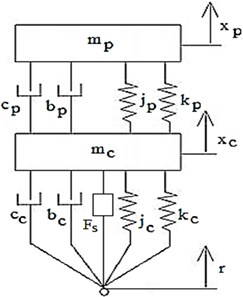
Hence the system was controlled in such a way so as to bring it back to this stable set of points when a disturbance was introduced. The designed controller would measure the displacement and would produce a force on mass instantaneously so that some vibration metrics were minimized. The three main performance metrics used in regular suspension design are passenger comfort, suspension deflection and road holding. This study focused on the first two. Fig. 2 shows non-linear coupled passenger car model with force actuator. With the addition of the controller force the equations were modified as:

8

{\dot{x}}_{1} = x_{2},

9

{\dot{x}}_{2} = \frac{- 1}{m_{p}} (k_{p} (x_{1} - x_{3}) + j_{p} {(x_{1} - x_{3})}^{3} {+ c}_{p} (x_{2} - x_{4}) + b_{p} {(x_{2} - x_{4})}^{3}),

10

{\dot{x}}_{3} = x_{4},

11

{\dot{x}}_{4} = {\frac{1}{m_{c}} (k}_{p} (x_{p} - x_{c}) + j_{p} {(x_{p} - x_{c})}^{3} + c_{p} ({\dot{x}}_{p} {- \dot{x}}_{c}) + b_{p} {({\dot{x}}_{p} - {\dot{x}}_{c})}^{3} - k_{c} (x_{c} - r)

- j_{c} {(x_{c} - r)}^{3} - c_{c} ({\dot{x}}_{c} - \dot{r}) - b_{c} {({\dot{x}}_{c} - \dot{r})}^{3} + F_{s}) .

Fig. 2Non-linear coupled passenger car model with force actuator

The system was linearized about the fixed point $x_{1}^{*} = x_{2}^{*} = x_{3}^{*} = x_{4}^{*} = 0$ .

The linearized equations obtained through a Taylor series expansion about the point were the same as in equations except for the cubic terms. In state space representation, the linearized equations were:

12

x_{1} = x_{p}, x_{2} = {\dot{x}}_{p}, x_{3} = x_{c}, x_{4} = {\dot{x}}_{c},

[\begin{matrix} {\dot{x}}_{1} \\ \dot{x_{2}} \\ \dot{x_{3}} \\ \dot{x_{4}} \end{matrix}] = [\begin{matrix} 0 & 1 & 0 & 0 \\ - \frac{k_{p}}{m_{p}} & - \frac{c_{p}}{m_{p}} & \frac{k_{p}}{m_{p}} & \frac{c_{p}}{m_{p}} \\ 0 & 0 & 0 & 1 \\ \frac{k_{p}}{m_{c}} & \frac{c_{p}}{m_{c}} & - \frac{{(k}_{p} + k_{c})}{m_{c}} & - \frac{{(c}_{p} + c_{c})}{m_{c}} \end{matrix}] [\begin{matrix} x_{1} \\ x_{2} \\ x_{3} \\ x_{4} \end{matrix}]

+ [\begin{matrix} 0 & 0 & 0 \\ 0 & 0 & 0 \\ 0 & 0 & 0 \\ \frac{k_{c}}{m_{c}} & \frac{c_{c}}{m_{c}} & \frac{1}{m_{c}} \end{matrix}] [\begin{matrix} r \\ \dot{r} \\ F_{s} \end{matrix}] .

3. Controller design

3.1. PID controller

A proportional-integral-derivative controller (PID controller) is a control loop feedback mechanism (controller) widely used in industrial control. A PID controller calculates an ”error” value as the difference between a measured process variable and a desired set-point, as shown in Fig. 3. The controller attempts to minimize the error in outputs by adjusting the process control inputs.

The PID controller algorithm involves three separate constant parameters, and is accordingly sometimes called three-term control: the proportional, the integral and derivative values, denoted P, I, and D. Simply put, these values can be interpreted in terms of time: P depends on the present error, I on the accumulation of past errors, and D is a prediction of future errors, based on current rate of change. The weighted sum of these three actions is used to adjust the process via a control element such as the position of a control valve, a damper:

13

u (t) = M V (t) = K_{p} e (t) + K_{i} \int_{0}^{t} e (τ) d τ + K_{d} \frac{d}{d t} e (t),

where $K_{p}$ – proportional gain, a tuning parameter, $K_{i}$ – integral gain, a tuning parameter, $K_{d}$ – derivative gain, a tuning parameter, $r (t)$ – reference signal, $c (t)$ – controlled output, $e (t)$ – error $= r (t) - c (t)$ , $t$ – instantaneous time (the present), $τ$ – variable of integration.

Fig. 3Block diagram of closed loop system

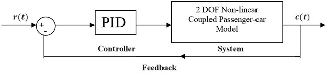
Fig. 4Block diagram of PID controller in Simulink

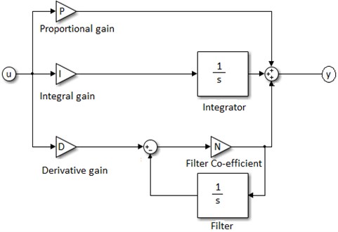
Simulations of the system were done in Simulink by modeling plant using MATLAB embedded function using Eqs. (8), (9), (10) and (11). The block diagram of PID controller in Simulink is as shown in Fig. 4. PID transfer function is given by:

14

T F = P + I (\frac{1}{s}) + D \frac{N f}{1 + N f (\frac{1}{s})} .

3.2. PID tuning

The system was simulated using the parameters mentioned in section 2. For controller synthesis, PID tuning was done using auto-tune option in Simulink and the values of the gain terms are given in Table 1. With these values of gain, the stability of the closed loop system was verified using root locus [37-38].

Table 1PID values generated in Simulink

PID values passenger acceleration controller
P	3197.515
I	16760.819
D	20.258
Nf (Filter coefficient)	150.027

3.3. H-∞ controller

H-∞ methods are used in control theory to synthesize controllers achieving stabilization with guaranteed performance. To use H-∞ methods, a control designer expresses the control problem as a mathematical optimization problem and then finds the controller that solves this optimization. H-∞ techniques have the advantage over classical control techniques in that they are readily applicable to problems involving multivariate systems with cross-coupling between channels; disadvantages of H-∞ techniques include the level of mathematical understanding needed to apply them successfully and the need for a reasonably good model of the system to be controlled. It is important to keep in mind that the resulting controller is only optimal with respect to the prescribed cost function and does not necessarily represent the best controller in terms of the usual performance measures used to evaluate controllers such as settling time, energy expended, etc. Also, non-linear constraints such as saturation are generally not well-handled.

The block diagram of closed loop with controller and weighting functions is as per Fig. 5. The measured output or feedback signal was ${\ddot{x}}_{p}$ . The controller was to act on this signal to produce the control input to the suspension model. The block $W_{n}$ served to model the sensor noise while measurement. $W_{r e f}$ was used to model the road disturbances. The block $W_{a c t}$ regulated the magnitude and frequency content of the force. The purpose of $W_{x 1}$ was to keep the acceleration transfer function small over the required frequency ranges.

Fig. 5Block diagram of closed loop with controller and weighting functions

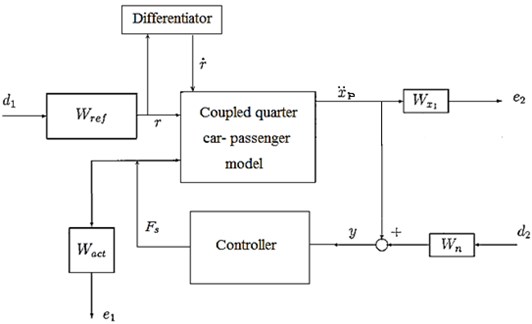
Controller is designed in MATLAB using Eq. (12). We chose the following weighting functions for simulation [14]:

W_{n} = 0.01, W_{r e f} = 0.15, W_{a c t} = \frac{1}{1500} \frac{(s + 10)}{(s + 100)}, W_{x 1} = \frac{1200}{s + 120} .

4. Results

In this section, simulation results for quarter car suspension system are given for the following cases:

1. Passive suspension;

2. With PID control;

3. With H-∞ control.

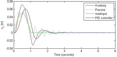
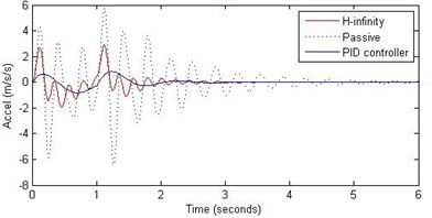
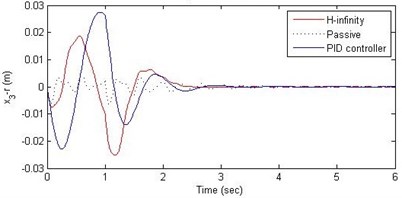
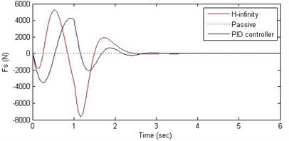
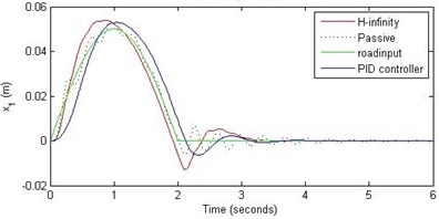
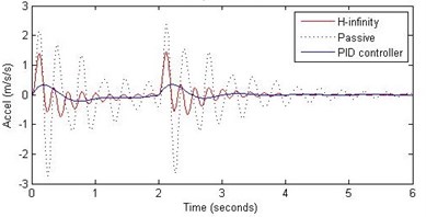
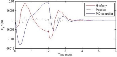
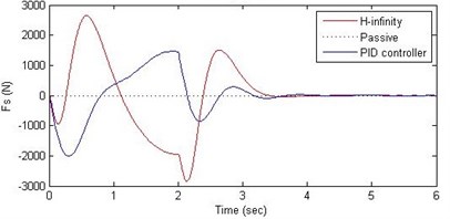
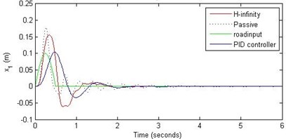
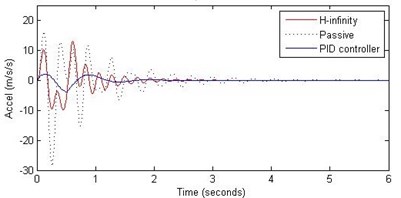
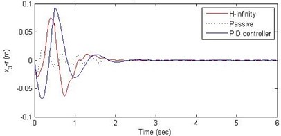
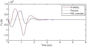
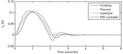
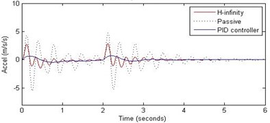
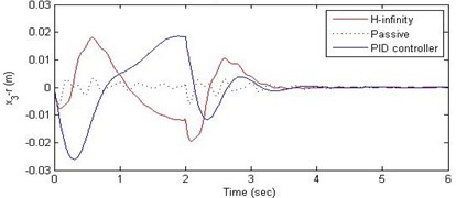
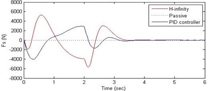
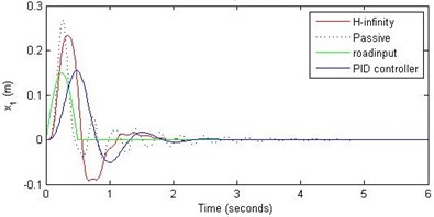
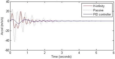
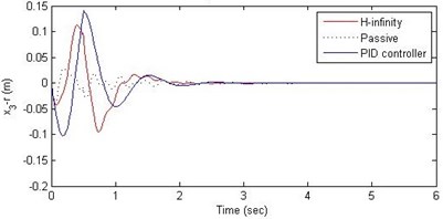
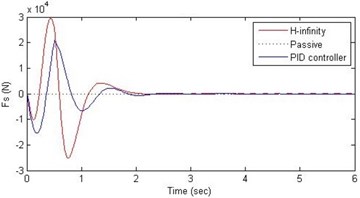
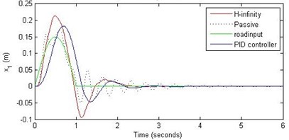
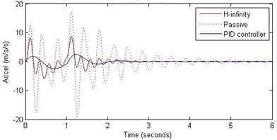
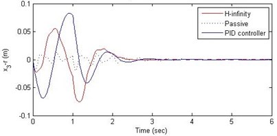
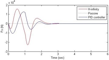
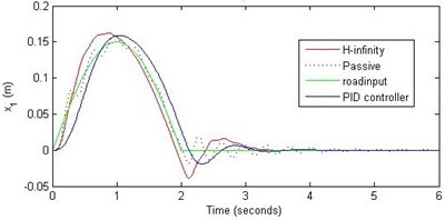
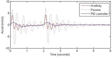
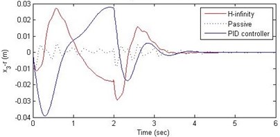
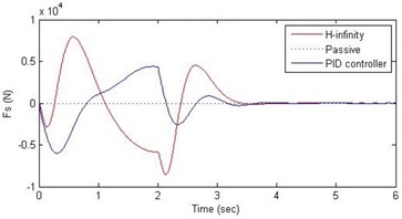
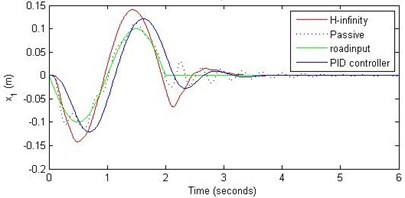
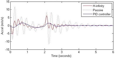
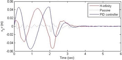
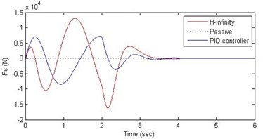
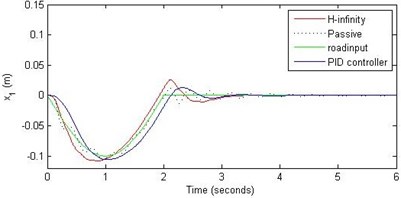
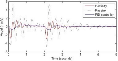
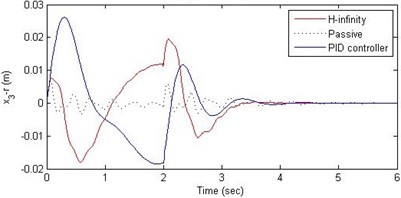
Fig. 6Comparison of different parameters with two controllers PID (blue) and H-∞ (red) with road input (green) as a bump with frequency 2π and amplitude 5 cm

Comparison of different parameters with two controllers PID (blue) and H-∞ (red) with road input (green) as a bump with frequency 2π and amplitude 5 cm

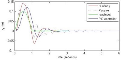
a) Passenger travel

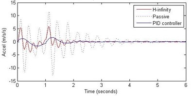
b) Passenger acceleration

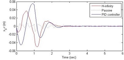
c) Suspension deflection

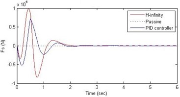
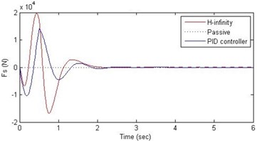
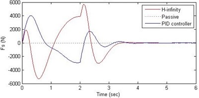
d) Damping force

Fig. 7Comparison of different parameters with two controllers PID (blue) and H-∞ (red) with road input (green) as a bump with frequency π and amplitude 5 cm

Comparison of different parameters with two controllers PID (blue) and H-∞ (red) with road input (green) as a bump with frequency π and amplitude 5 cm

a) Passenger travel

b) Passenger acceleration

c) Suspension deflection

d) Damping force

The road disturbance is considered to be half-sinusoidal wave, having different height and width as specified by green colors in Figs. 6-14. This particular shape faithfully mimics the actual road disturbance. We have taken the following cases: sinusoidal wave having $π /$ 2, $π$ and 2 $π$ rad/sec of frequency and amplitudes of 5, 10 and 15 cm. Performance of both the control schemes and the passive suspension is evaluated for all these cases of road disturbance inputs. Further, two more road disturbance inputs are considered: Fig. 15, a pothole of 10 cm shown by green color and in Fig. 16, a full sine wave (one complete cycle) of 10 cm of amplitude and $π$ rad/s frequency is shown by green color. In all the cases the passenger displacement, passenger acceleration, suspension deflection and the actuator force are plotted against time. Graphical results are shown below in Fig. 6 through Fig. 16 for the different road disturbance cases.

Fig. 8Comparison of different parameters with two controllers PID (blue) and H-∞ (red) with road input (green) as a bump with frequency π/2 and amplitude 5 cm

Comparison of different parameters with two controllers PID (blue) and H-∞ (red) with road input (green) as a bump with frequency π/2 and amplitude 5 cm

a) Passenger travel

b) Passenger acceleration

c) Suspension deflection

d) Damping force

Fig. 9Comparison of different parameters with two controllers PID (blue) and H-∞ (red) with road input (green) as a bump with frequency 2π and amplitude 10 cm

Comparison of different parameters with two controllers PID (blue) and H-∞ (red) with road input (green) as a bump with frequency 2π and amplitude 10 cm

a) Passenger travel

b) Passenger acceleration

c) Suspension deflection

d) Damping force

For the case of sinusoidal road disturbance we find that there is no significant improvement in the passenger displacement in the PID control and H-∞ control over the passive suspension. Rather, in certain cases we find the passenger deflection to be marginally increased in the two control schemes when compared with the passive suspension.

However, the passenger acceleration (m/s²) is reduced by a significant proportion thereby increasing the passenger comfort in all the cases. For example:

1. $π /$ 2 rad/s and 5 cm height: the passenger acceleration is found to be in the range of –2.8 to 2.3 (passive suspension), –0.22 to 0.35 (PID) and –0.8 to 1.5 (H-∞).

2. $π$ rad/s and 10 cm height: the passenger acceleration is found to be in the range of –13 to 12 (passive suspension), –1.7 to 1.7 (PID) and –4 to 5 (H-∞).

3. 2 $π$ rad/s and 15 cm height: the passenger acceleration is found to be in the range of –40 to 25 (passive suspension), –5.7 to 3 (PID) and –18 to 19 (H-∞).

Fig. 10Comparison of different parameters with two controllers PID (blue) and H-∞ (red) with road input (green) as a bump with frequency π and amplitude 10 cm

Comparison of different parameters with two controllers PID (blue) and H-∞ (red) with road input (green) as a bump with frequency π and amplitude 10 cm

a) Passenger travel

b) Passenger acceleration

c) Suspension deflection

d) Damping force

Fig. 11Comparison of different parameters with two controllers PID (blue) and H-∞ (red) with road input (green) as a bump with frequency π/2 and amplitude 10 cm

Comparison of different parameters with two controllers PID (blue) and H-∞ (red) with road input (green) as a bump with frequency π/2 and amplitude 10 cm

a) Passenger travel

b) Passenger acceleration

c) Suspension deflection

d) Damping force

Further, we notice that the PID control gives improved passenger acceleration when compared with the H-∞ control for the given tuning. In all the cases we observe that the suspension deflection is minimum for the passive suspension system as opposed to that for the other two control schemes for the same road disturbance input. When compared between the PID and H-∞ control, the suspension deflection is found to be on higher side in case of the H-∞ control keeping the road disturbance the same. Accordingly, we notice that the control effort or the actuator force (kN) is on higher side for the H-∞ control when compared with that of the PID control for the same road disturbance. There is marginal improvement in terms of the settling time in the two control schemes when compared with the passive system for each of the road disturbance input. However, the settling time is almost equal for both the control schemes for a given road disturbance.

Fig. 12Comparison of different parameters with two controllers PID (blue) and H-∞ (red) with road input (green) as a bump with frequency 2π and amplitude 15 cm

Comparison of different parameters with two controllers PID (blue) and H-∞ (red) with road input (green) as a bump with frequency 2π and amplitude 15 cm

a) Passenger travel

b) Passenger acceleration

c) Suspension deflection

d) Damping force

Fig. 13Comparison of different parameters with two controllers PID (blue) and H-∞ (red) with road input (green) as a bump with frequency π and amplitude 15 cm

Comparison of different parameters with two controllers PID (blue) and H-∞ (red) with road input (green) as a bump with frequency π and amplitude 15 cm

a) Passenger travel

b) Passenger acceleration

c) Suspension deflection

d) Damping force

Fig. 14Comparison of different parameters with two controllers PID (blue) and H-∞ (red) with road input (green) as a bump with frequency π/2 and amplitude 15 cm

Comparison of different parameters with two controllers PID (blue) and H-∞ (red) with road input (green) as a bump with frequency π/2 and amplitude 15 cm

a) Passenger travel

b) Passenger acceleration

c) Suspension deflection

d) Damping force

Fig. 15Comparison of different parameters with two controllers PID (blue) and H-∞ (red) with road input (green) as a continuous pothole and bump with frequency π and amplitude 10 cm

Comparison of different parameters with two controllers PID (blue) and H-∞ (red) with road input (green) as a continuous pothole and bump with frequency π and amplitude 10 cm

a) Passenger travel

b) Passenger acceleration

c) Suspension deflection

d) Damping force

5. Conclusions

In this paper, we presented design of suspension system for a 2DOF quarter car system using nonlinear model. Two different control schemes, PID control and H-∞ control, were used to design the controller. A comparative study of these two methods and of the passive suspension system was presented through simulations. In order to assess the passenger comfort, we considered the time variation of passenger displacement and passenger acceleration, when subjected to a family of road disturbances. In this study it was found that both the control schemes do not offer any significant advantage over the passive suspension when it comes to passenger displacement. However, the passenger comfort is improved by a great amount in these two control schemes in the sense that, both the control schemes reduce the range of passenger acceleration. Further, the PID control scheme was found to perform better as compared to the H-∞ control scheme. Another aspect of the comparative study was related to the suspension deflection and the control effort. The passive suspension system gave minimum suspension deflection when compared with the other two control methods. The suspension deflection is more in the H-∞ control than that of in the PID control. Accordingly, the control effort (in terms of the maximum and minimum of the force) was found to be more in the H-∞ control as compared with that in the PID control scheme.

Fig. 16Comparison of different parameters with two controllers PID (blue) and H-∞ (red) with road input (green) as a pothole with frequency π/2 and amplitude 10 cm

Comparison of different parameters with two controllers PID (blue) and H-∞ (red) with road input (green) as a pothole with frequency π/2 and amplitude 10 cm

a) Passenger travel

b) Passenger acceleration

c) Suspension deflection

d) Damping force

References

Guglielmino E., Sireteanu T., Stammers C. W., Ghita G., Giuclea M. Semi-active suspension control. Springer, 2008.

Search CrossRef
Mouleeswaran Senthilkumar Design and Development of PID Controller-Based Active Suspension System for Automobiles, PID Controller Design Approaches – Theory, Tuning and Application to Frontier Areas. Dr. Marialena Vagia (Ed.), 2012.

Search CrossRef
GillespieT. D. Fundamentals of Vehicle Dynamics. Society of Automotive Engineers, Warrendale, USA, 1992.

Search CrossRef
Federspiel-Labrosse G. M. Contribution to the study and analysis of the suspension of vehicles. Journal de la SIA, FISITA, 1954, p. 427-436, (in French).

Search CrossRef
Elbeheiry E. M., Bode O., Cho D. Advanced ground vehicle suspension systems. Vehicle System Dynamics, Vol. 24, 1995, p. 231-258.

Search CrossRef
Hedrick J. K., Wormely D. N. Active suspension for ground support transportation. ASME AMD, Vol. 15, 1975, p. 21-40.

Search CrossRef
Sharp R. S., Crolla D. A. Road vehicle suspension system design. Vehicle System Dynamics, Vol. 16, Issue 3, 1987, p. 167-192.

Search CrossRef
Karnopp D. C. Active and semi-active vibration isolation. Journal of Mechanical Design, Vol. 117, 1995, p. 177-185.

Search CrossRef
Hrovat D. Survey of advanced suspension development and related optimal control application. Automatica, Vol. 30, Issue 10, 1997, p. 1781-1817.

Search CrossRef
Elmadany M. M., Abduljabbar Z. S. Linear quadratic Gaussian control of a quarter-car suspension. Vehicle System Dynamics, Vol. 32, Issue 6, 1999, p. 479-497.

Search CrossRef
Al-Holou N., Lahdhiri T., Joo D., Weaver J., Al-Abbas F. Sliding mode neural network inference fuzzy logic control for active suspension systems. IEEE Transactions on Fuzzy Systems, Vol. 10, Issue 2, 2002, p. 234-246.

Search CrossRef
Fialho I., Balas G. J. Design of nonlinear controllers for active vehicle suspensions using parameter varying control synthesis. Vehicle System Dynamics, Vol. 33, Issue 5, 2000, p. 351-370.

Search CrossRef
Yamashita M., Fujimori K., Hayakawa K., Kimura H. Application of H-infinity control to active suspension systems. Preprint of the 12th IFAC World Congress, Sydney, Vol. 3, 1993, p. 143-146.

Search CrossRef
Karlsson N., Dahleh M., Hrovat D. Nonlinear H control of active suspensions. Proceedings of the American Control Conference, Arlington, VA, 2001, p. 3329-3334.

Search CrossRef
Fialho I., Balas G. J. Road adaptive active suspension design using linear parameter-varying gainscheduling. IEEE Transactions on Control Systems Technology, Vol. 10, Issue 1, 2002, p. 43-54.

Search CrossRef
Thompson A., Pearce C. Performance index for a preview active suspension applied to a quarter-car model. Vehicle System Dynamics, Vol. 35, Issue 1, 2001, p. 55-66.

Search CrossRef
Suggs C. W., Abrams C. F., Stikeleather L. F. Application of a damped spring-mass human vibration simulator in vibration testing of vehicle seats. Ergonomics, Vol. 12, 1969, p. 79-90.

Search CrossRef
Muksian R., Nash C. D. A model for the response of seated humans to sinusoidal displacements of the seat. Journal of Biomechanics, Vol. 7, 1974, p. 209-215.

Search CrossRef
Pope M. H., Wilder D. G., Jorneus L., Broman H., Svensson M., Andersson G. The response of the seated human to sinusoidal vibration and impact. Journal of Biomechanical Engineering, Vol. 109, 1987, p. 279-284.

Search CrossRef
Griffin M. J., Whitham E. M., Parsons K. C. Vibration and comfort. Part I: Translational seat vibration. Ergonomics, Vol. 25, 1982, p. 603-630.

Search CrossRef
Pope M. H., Broman H., Hansson T. The dynamic response of a subject seated on various cushions. Ergonomics, Vol. 32, 1989, p. 1155-1166.

Search CrossRef
Zimmermann C. L., Cook T. M. Effects of vibration frequency and postural changes on human responses to seated whole-body vibration exposure. International Archives of Occupational and Environmental Health, Vol. 69, 1997, p. 165-179.

Search CrossRef
Wilder D., Magnusson M. L., Fenwick J., Pope M. The effect of posture and seat suspension design on discomfort and back muscle fatigue during simulated truck driving. Applied Ergonomics, Vol. 25, 1994, p. 66-76.

Search CrossRef
Cho Y., Yoon Y.-S. Biomechanical model of human on seat with backrest for evaluating ride quality. International Journal of Industrial Ergonomics, Vol. 27, 2001, p. 331-345.

Search CrossRef
Lewis C. H., Griffin M. J. The transmission of vibration to the occupants of a car seat with a suspended back-rest. Proceedings of the Institution of Mechanical Engineers, Part D – Journal of Automobile Engineering, Vol. 210, 1996, 199-207.

Search CrossRef
Wan Y., Schimmels J. M. Optimal seat suspension design based on minimum simulated subjective response. Journal of Biomechanical Engineering, Vol. 119, 1997, p. 409-416.

Search CrossRef
Fritz M. Estimation of spine forces under whole-body vibration by means of a biomechanical model and transfer functions. Aviation, Space, and Environmental Medicine, Vol. 68, 1997, p. 512-519.

Search CrossRef
Kumar A., Varghese M., Mohan D., Mahajan P., Gulati P., Kale S. Effect of whole-body vibration on the lower back – a study of tractor-driving farmers in North India. SPINE, Vol. 24, 1999, p. 2506-2515.

Search CrossRef
Verver M. M., van Hoof J., Oomens C. W. J., van de Wouw N., Wismans J. S. H. M. Estimation of spinal loading in vertical vibrations by numerical simulation. Clinical Biomechanics, Vol. 18, 2003, p. 800-811.

Search CrossRef
Harrison D. D., Harrison S. O., Croft A. C., Harrison D. E., Troyanovich S. T. Sitting biomechanics. Part II: Optimal car driver’s seat and optimal driver’s spinal model. Journal of Manipulative and Physiological Therapeutics, Vol. 23, 2000, p. 37-47.

Search CrossRef
Papalukopoulos C., Natsiavas S. Nonlinear biodynamics of passengers coupled with quarter car models. Journal of Sound and Vibrations, Vol. 304, 2007, p. 50-71.

Search CrossRef
Liang C. C., Chaing C. F. A study on biodynamic models of seated human subjects exposed to vertical vibrations. International Journal of Industrial Ergonomics, Vol. 36, 2006, p. 869-890.

Search CrossRef
Hinz B., Seidel H. The non-linearity of the human body’s response during sinusoidal whole body vibration. Industrial Health, Vol. 25, 1987, p. 169-181.

Search CrossRef
Chantranuwathana S., Peng H. Adaptive robust force control for vehicle active suspensions. International Journal of Adaptive Control and Signal Processing, Vol. 18, 2004, p. 83-102.

Search CrossRef
Gaspar P., Sazaszi I., Bokor J. Active suspension design using linear parameter varying control. International Journal of Vehicle Autonomous Systems, Vol. 1, Issue 2, 2003, p. 206-221.

Search CrossRef
Anilkumar Allen Hysteretic Seat Design and Control of Passenger Vibrations in a Quarter Car Model. M.E. dissertation, BITS Pilani, K. K. Birla Goa campus, India, 2012.

Search CrossRef
Mathworks, Matlab and Simulink tutorials, www.mathworks.com.

Search CrossRef
Ogata Katsuhiko Modern Control Systems. 5th Edition. Prentice Hall, 2010.

Search CrossRef
Lauwerys Christophe, Swevers Jan, Sas Paul Robust linear control of an active suspension on a quarter car test-rig. Elsevier Control Engineering Practice, Vol. 13, 2005, p. 577-586.

Search CrossRef

About this article

Received

28 June 2014

Accepted

19 November 2014

Published

30 December 2014

Keywords

quarter car model

PID controller

H-infinity controller

This is an open access article distributed under the Creative Commons Attribution License, which permits unrestricted use, distribution, and reproduction in any medium, provided the original work is properly cited.