Passive fault-tolerant control for vehicle active suspension system based on H2/H∞ approach

In this paper, a robust passive fault-tolerant control (RPFTC) strategy based on $H_{2} / H_{\infty}$ approach and an integral sliding mode passive fault tolerant control (ISMPFTC) strategy based on $H_{2} / H_{\infty}$ approach for vehicle active suspension are presented with considering model uncertainties, loss of actuator effectiveness and time-domain hard constraints of the suspension system. $H_{\infty}$ performance index less than $γ$ and $H_{2}$ performance index is minimized as the design objective, avoid choosing weighting coefficient. The half-car model is taken as an example, the robust passive fault-tolerant controller and the integral sliding mode passive fault tolerant control law is designed respectively. Three different fault modes are selected. And then compare and analyze the control effect of vertical acceleration of the vehicle body and pitch angular acceleration of passive suspension control, robust passive fault tolerant control and integral sliding mode passive fault tolerant control to verify the feasibility and effectiveness of passive fault tolerant control algorithm of active suspension. The studies we have performed indicated that the passive fault tolerant control strategy of the active suspension can improve the ride comfort of the suspension system.

Passive fault-tolerant control for vehicle active suspension system based on H2/H∞ approach

Highlights

Actuator partial failure, time-domain hard constraints and model uncertainties are considered.
Two passive fault-tolerant control strategy based on H2/H∞ approach are proposed.
The proposed two control strategies can improve the ride comfort of the vehicle.

1. Introduction

A suspension system is a very important component of any vehicle. It flexibly connects the vehicle body and the axles, carries the vehicle body; transmits all vertical forces between body and road, including bears the forces between the tires and body, absorbs the shock from the road surface; protects the vehicle from unwanted vibrations and avoids excessive suspension stroke or related hard stop/impact. The suspension plays a key role in the riding comfort and handling stability [1-3]. The primary functions of a vehicle suspension system are to isolate a car body from road disturbances in order to provide good ride quality, to keep good road holding, to provide good handling and support the vehicle static weight [4, 5]. Suspensions generally fall into either of two groups-dependent suspensions and independent suspensions. Suspension systems can be divided into passive suspension, semi-active suspension, and active suspension, according to the different control modes used [1]. There are generally three fundamental elements for a typical vehicle suspension system, including springing, damping, and location of the wheel [6]. Active suspension system contains separate actuator that is able to provide external forces to both add and dissipate energy from the system. The task of the suspension spring is to carry the body mass and to isolate the body from road disturbances. The suspension damper contributes to both driving safety and quality. Its task is the damping of body and wheel oscillations. A non-bouncing wheel is a condition for transferring road-contact forces [2].

However, conventional suspensions can achieve a trade-off between ride comfort and road holding since their spring and damping coefficients cannot be adaptively tuned according to driving efforts and road conditions. They can achieve good ride comfort and road holding only under the designed conditions [7]. Active suspension systems have the best potential to deal with conflicting objectives placed on a suspension system a potential to deal with the trade-off between the conflicting suspension performance measures. Because vehicle active suspension can significantly improve the ride comfort of passengers, meet the requirements of handling stability simultaneously. Over the past three decades, many researchers have devoted themselves to the theory and simulation studies on the control method of vehicle active suspension. Many advances have been made in active suspension and control theory nowadays.

The active suspension control problem can be considered as a disturbance attenuation problem with time-domain hard constraints [8, 9]. The mixed $H_{2} / H_{\infty}$ guaranteed cost control problem of state feedback control laws is considered in [10] for linear systems with norm-bounded parameter uncertainty. The $H_{\infty}$ state feedback control strategy with time domain hard constraints was proposed under non-stationary running [11]. [12] designed a linear, robust, guaranteed-cost state feedback control with pole region constraints subject to active suspension system uncertainties. By the LMI (Linear Matrix Inequalities) method, a convex optimization problem is formulated to find the corresponding controller. A 3 DOF quarter car model is used in [13]. LQR based fuzzy controller; Fuzzy PID controller and Linear Quadratic Controller (LQR) are designed respectively to analyze and compare the performance characteristics of the active system with the uncontrolled system or passive suspension system. In [14], a robust model predictive control algorithm for polytopic uncertain systems with time-varying delays is presented for active suspension systems. However, most often, controllers are designed for the faultless suspension system so that the closed loop meets given performance specifications in studies of active suspension. Since not taking full account of the suspension system may exist malfunctions such as actuators, sensors or model parameters, which may lead to a degraded system performance (unsatisfactory performance) or even the loss of the system function (even instability) [15]. That is to say, once an actuator or a sensor fault occurs in a suspension system, the conventional controllers cannot achieve better performance in comparison with the reliable and fault-tolerant controllers.

Fault tolerant control systems (FTCS) as control systems that possess the ability to accommodate system component failures automatically. They are capable of maintaining overall system stability and acceptable performance in the event of such failures. FTCS were also known as self-repairing, reconfigurable, restructurable, or self designing control systems [17-19]. Generally speaking, fault tolerant control can be classified into two types: active fault tolerant control (AFTC) and passive fault tolerant control (PFTC). AFTC reacts to the system component failures actively, by means of a fault detection and diagnosis (FDD) component that detects, isolates, and estimates the current faults, and re-configuring on-line the controller, so that the stability and acceptable performance of the entire system can be maintained [18, 19]. Robust control is closely related to passive fault tolerant control systems (PFTCS). The controller is designed to be robust against disturbances and uncertainty during the design stage. That is, controllers are designed to be robust against a class of presumed fault. In other words, the starting point of the design is to reduce system dependency on the operation of a single component, even in the case of such failures and no correction, the system can still maintain some “acceptable” level of performance or degrade gracefully [17]. This enables the controller to counteract the effect of a fault without requiring reconfiguration or fault detection and isolation(FDI). Passive schemes operate independently of any fault information and basically exploit the robustness of the underlying controller. Such a controller is usually less complex, but in order to cope with ‘worst case’ fault effects, has a certain degree of conservatism [16, 18, 19]. However, its advantages are obvious: the parameters and structure of the controller are to be designed fixed; it neither needs to adjust the control law and control parameters online, nor needs fault detection, diagnosis and isolation; it is easy to realize and has the advantage of avoiding the time delay, which is very important [20-22].

A passive fault-tolerant $H_{\infty}$ controller is designed in [23] such that the resulting control system is reliable since it has the capability of guaranteeing asymptotic stability and $H_{\infty}$ performance, and simultaneously satisfying the constraint performance in the scenarios of actuator failures. In [24], a fault-tolerant control approach is proposed to deal with the problem of fault accommodation for unknown actuator failures of active suspension systems, where an adaptive robust controller is designed to adapt and compensate the parameter uncertainties, external disturbances and uncertain non-linearities generated by the system itself and actuator failures. In [25], the robust fault-tolerant $H_{\infty}$ control problem of active suspension systems with finite-frequency constraint is investigated. Both the actuator faults and external disturbances are considered in the controller synthesis. Other performances such as suspension deflection and actuator saturation are also considered. In [26], an adaptive fault tolerant control problem for half-car active suspension system subject to Markovian jumping actuator failures is considered. By employing adaptive backstepping technique, a new adaptive fault tolerant control scheme is proposed, which ensures the boundedness in probability of the considered systems.

Sliding mode based control schemes are a strong candidate for fault tolerant control because of their inherent robustness to matched uncertainties. Actuator faults can be effectively modeled as matched uncertainties and therefore sliding mode based control schemes have an inherent capability to directly deal with actuator faults [27]. In [28], a new robust strategy is presented which utilized the proportional-integral sliding mode control scheme. In [29] a sliding mode control is designed for a full nonlinear vehicle active suspension system. Sensor faults effects on the behavior of the controlled system are analyzed and a fault tolerant control strategy to compensate for the sensor faults is proposed. [30] presents adaptive sliding mode fault tolerant control for magneto-rheological (MR) suspension system considering the partial fault of MR dampers. In [31], an adaptive proportional-integral-derivative (PID) controller is proposed. Designing an adaptation scheme for the PID gains to accommodate actuator faults. A fault tolerant control approach based on a novel sliding mode method is proposed in [32] for a full vehicle suspension system aims at retaining system stability in the presence of model uncertainties, actuator faults, parameter variations.

This paper is based on the previous research results, consider that the vehicle active suspension system off-line designed controller in the event of malfunctions in actuators and model uncertainties cannot achieve the desired control effect, and even controller appear failure make the suspension system loss of stability. In view of this, under the premise of fully taken into account the time domain hard constraints of the suspension system; for the half-car active suspension system with actuator faults and model uncertainties, a robust passive fault tolerant control scheme based on $H_{2} / H_{\infty}$ approach and an integral sliding mode passive fault tolerant control scheme based on $H_{2} / H_{\infty}$ approach is designed respectively.

2. Half-car model

Vehicle vibration models can be divided into quarter-car model, half-car model, full-car model. The quarter-vehicle model was initially developed to explore active suspension capabilities and gave birth to the concepts of skyhook damping and fast load leveling, which are now being developed toward actual, large-scale production applications. The quarter-car model has been the bench model used in the study of control algorithm for intelligent suspension system. Although the model is very simple and is considering only vertical vibration motions of the sprung mass and the unsprung mass, it is very useful in initial development. By considering the vertical dynamics and taking into account the vehicle’s symmetry, a suspension can be reduced to the quarter-car model. To account for the pitch motion or roll motion, a half-car model is adopted by many researchers. The model is considering the vertical vibration and pitch motions of vehicle body, and the vertical motion of front and rear wheels. The half-car model was represented to simulate ride characteristics of a simplified whole vehicle, which leads to significant improvement in ride and handling. The vehicle body of the full-car model is assumed to be rigid and has seven degree-of-freedom in heave, pitch, and roll directions [7].

A four degree-of-freedom half-car model is shown in Fig. 1. The model can simultaneously represent the passive suspension and active/semi-active according to the state of the actuator. If the actuator is neglected, the model is a passive suspension. The model is an active suspension if the actuator can generate active control forces, while the model is a semi-active suspension if the actuator can provide only damping forces. The model has been used extensively in the literature and captures many important characteristics of vertical and pitch motions.

Fig. 1Model of half-car active suspension system

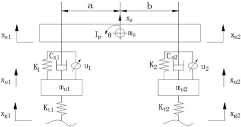
The half-car model is shown in Fig. 1. With the assumption of a small pitch angle $θ$ , $s i n θ \approx θ$ , we have the following approximate linear relationships:

{x_{s 1} = x}_{s} - a θ, {x_{s 2} = x}_{s} + b θ, θ = \frac{{(x}_{s 2} - x_{s 1})}{(a + b)} .

The dynamic equations of this model can be written as:

1

\{\begin{array}{l} {m_{u 1} {\ddot{x}}_{u 1} = K_{t 1} (x_{g 1} - x_{u 1}) - K_{1} (x_{u 1} - x_{s 1}) - C_{s 1} ({\dot{x}}_{u 1} - {\dot{x}}_{s 1}) - u}_{1}, \\ {m_{u 2} {\ddot{x}}_{u 2} = K_{t 2} (x_{g 2} - x_{u 2}) - K_{2} (x_{u 2} - x_{s 2}) - C_{s 2} ({\dot{x}}_{u 2} - {\dot{x}}_{s 2}) - u}_{2}, \\ I_{p} \ddot{θ} = - a K_{1} (x_{u 1} - x_{s 1}) + b K_{2} (x_{u 2} - x_{s 2}) - a C_{s 1} ({\dot{x}}_{u 1} - {\dot{x}}_{s 1}) \\ + b C_{s 2} ({\dot{x}}_{u 2} - {\dot{x}}_{s 2}) - a u_{1} + b u_{2}, \\ m_{s} {\ddot{x}}_{s} = K_{1} (x_{u 1} - x_{s 1}) + K_{2} (x_{u 2} - x_{s 2}) + C_{s 1} ({\dot{x}}_{u 1} - {\dot{x}}_{s 1}) + C_{s 2} ({\dot{x}}_{u 2} - {\dot{x}}_{s 2}) + u_{1} + u_{2}, \\ x_{s 1} = x_{s} - a θ, \\ x_{s 2} = x_{s} + b θ, \end{array}

where $m_{u 1}$ , $m_{u 2}$ are the front and rear unsprung mass respectively; $I_{p}$ is pitch moment of inertia; $θ$ represents the pitch angular; $m_{s}$ is the sprung mass; $K_{1}$ and $K_{2}$ are the stiffness coefficient of front and rear suspension respectively; $C_{s 1}$ and $C_{s 2}$ are the damping coefficient of front and rear suspension respectively; $a$ and $b$ are the distance of front and rear axle to sprung mass center of gravity respectively; $u_{1}$ and $u_{2}$ are actuator control output force of the front and rear suspension respectively; $x_{u 1}$ and $x_{u 2}$ are the displacements of the front and rear unsprung mass respectively; $x_{g 1}$ and $x_{g 2}$ are the road profile inputs of the front and rear suspension system respectively.

Taking into account the time domain hard constraints on the suspension system [8, 9], it is necessary to keep suspension dynamic displacement in the usable range, so as to avoid bumping the limit blocks:

2

|x_{s i} - x_{u i}| < S_{m a x}, (i = 1, 2),

where $S_{m a x}$ is the maximum suspension deflection.

Consider that the driving stability of the vehicle requirements, the dynamic tyre load doesn’t exceed the static tyre load in order to ensure the tire's grip capacity:

3

|K_{t i} {(x}_{u i} - x_{g i})| < (m_{s i} + m_{u i}) g, (i = 1, 2),

where $m_{s 1}$ , $m_{s 2}$ are the static load mass of the front and rear suspension parts respectively.

The active control force provided for the active suspension system should be confined to a certain range prescribed by limited power of the actuator:

4

|u_{i}| \leq F_{m a x}, (i = 1, 2),

where $F_{m a x}$ represents actuator output threshold.

Generally speaking, $H_{\infty}$ control strategy can solve the robust stability problem of a controlled target, and $H_{2}$ control strategy lets the controlled targets have a better dynamic performance. Combining on $H_{2} / H_{\infty}$ to build a hybrid control strategy, the problems of robust stability and optimal dynamic performance of a controlled target can be solved with better results. For a half-vehicle model, the riding comfort is related to the body vertical acceleration, pitching angular acceleration. The handling stability is related to the front and rear tyre dynamic loads. Based upon this consideration, and also considering how to reduce the complexity of a controller, a multi-objective optimization control strategy for an active suspension system is introduced. Choosing $H_{\infty}$ norm as the robust performance index of the time domain hard constraints, $H_{2}$ norm as the time-domain LQG performance index of perturbation action.

That is, the constrained output ( $Z_{\infty}$ ) and controlled output ( $Z_{2}$ ) are defined as follows:

5

\{\begin{matrix} Z_{\infty} = {[\frac{x_{s 1} - x_{u 1}}{S_{m a x}} \frac{x_{s 2} - x_{u 2}}{S_{m a x}} \frac{K_{t 1} (x_{u 1} - x_{g 1})}{(m_{s 1} + m_{u 1}) g} \frac{K_{t 2} {(x}_{u 2} - x_{g 2})}{(m_{s 2} + m_{u 2}) g} \frac{u_{1}}{F_{m a x}} \frac{u_{2}}{F_{m a x}}]}^{T}, \\ Z_{2} = {[{\ddot{x}}_{s} \ddot{θ}]}^{T}, \\ m_{s 1} = (\frac{b}{(a + b)}) m_{s} g, \\ m_{s 2} = {(\frac{a}{(a + b)}) m}_{s} g . \end{matrix}

The selected state vector $X = {[x_{s 1} - x_{u 1} x_{s 2} - x_{u 2} {\dot{x}}_{s 1} {\dot{x}}_{s 2} x_{u 1} - x_{g 1} x_{u 2} - x_{g 2} {\dot{x}}_{u 1} {\dot{x}}_{u 2}]}^{T}$ ; the road surface vertical speed ( ${\dot{x}}_{g 1}, {\dot{x}}_{g 2}$ ) are used as interference inputs, i.e. $W = [{\dot{x}}_{g 1}, {\dot{x}}_{g 2}]^{T}$ . Then the governing equations $σ_{f}$ can be presented in the following state-space form:

6

\{\begin{matrix} \dot{X} = A X + B_{1} W + B_{2} U, \\ Z_{\infty} = C_{1} X + D_{11} W + D_{12} U \\ Z_{2} = C_{2} X + D_{21} W + D_{22} U, \end{matrix},

where:

D_{11} = z e r o s (6,2), D_{21} = z e r o s (2), D_{12} = [\begin{matrix} 0 0 0 0 \frac{1}{F_{m a x}} 0 \\ 0 0 0 0 0 \frac{1}{F_{m a x}} \end{matrix}],

D_{22} = [\begin{matrix} \frac{1}{m_{s}} & \frac{1}{m_{s}} \\ \frac{- a}{I_{p}} & \frac{b}{I_{p}} \end{matrix}], {B_{1} = [\begin{matrix} 0 0 0 0 - 1 0 0 0 \\ 0 0 0 0 0 - 1 0 0 \end{matrix}]}_{2 \times 8},

B_{2} = [\begin{matrix} 0 0 \frac{1}{m_{s}} + \frac{a^{2}}{I_{p}} \frac{1}{m_{s}} - \frac{a b}{I_{p}} 0 0 \frac{- 1}{m_{u 1}} 0 \\ 0 0 \frac{1}{m_{s}} - \frac{a b}{I_{p}} \frac{1}{m_{s}} + \frac{b^{2}}{I_{p}} 0 0 0 \frac{- 1}{m_{u 1}} \end{matrix}],

A = {[\begin{matrix} 0 & 0 & 1 & 0 & 0 & 0 & - 1 & 0 \\ 0 & 0 & 0 & 1 & 0 & 0 & 0 & - 1 \\ \frac{- K_{1}}{m_{s}} - \frac{a^{2} K_{1}}{I_{p}} & \frac{- K_{2}}{m_{s}} + \frac{a b K_{2}}{I_{p}} & \frac{- C_{s 1}}{m_{s}} - \frac{a^{2} C_{s 1}}{I_{p}} & \frac{- C_{s 2}}{m_{s}} + \frac{a b C_{s 2}}{I_{p}} & 0 & 0 & \frac{C_{s 1}}{m_{s}} + \frac{a^{2} C_{s 1}}{I_{p}} & \frac{C_{s 2}}{m_{s}} + \frac{a b C_{s 2}}{I_{p}} \\ \frac{- K_{1}}{m_{s}} + \frac{a b K_{1}}{I_{p}} & \frac{- K_{2}}{m_{s}} - \frac{b^{2} K_{2}}{I_{p}} & \frac{- C_{s 1}}{m_{s}} + \frac{a b C_{s 1}}{I_{p}} & \frac{- C_{s 2}}{m_{s}} - \frac{b^{2} C_{s 2}}{I_{p}} & 0 & 0 & \frac{C_{s 1}}{m_{s}} + \frac{a b C_{s 1}}{I_{p}} & \frac{C_{s 2}}{m_{s}} + \frac{b^{2} C_{s 2}}{I_{p}} \\ 0 & 0 & 0 & 0 & 0 & 0 & 1 & 0 \\ 0 & 0 & 0 & 0 & 0 & 0 & 0 & 1 \\ \frac{K_{1}}{m_{u 1}} & 0 & \frac{C_{s 1}}{m_{u 1}} & 0 & \frac{- K_{t 1}}{m_{u 1}} & 0 & \frac{{- C}_{s 1}}{m_{u 1}} & 0 \\ 0 & \frac{K_{2}}{m_{u 2}} & 0 & \frac{C_{s 2}}{m_{u 2}} & 0 & \frac{- K_{t 2}}{m_{u 2}} & 0 & \frac{{- C}_{s 2}}{m_{u 2}} \end{matrix}]}_{8 \times 8},

C_{1} = {[\begin{matrix} \frac{1}{S_{m a x}} & 0 & 0 & 0 & 0 & 0 & 0 & 0 \\ 0 & \frac{1}{S_{m a x}} & 0 & 0 & 0 & 0 & 0 & 0 \\ 0 & 0 & 0 & 0 & \frac{K_{t 1}}{m_{s 1} g + m_{u 1} g} & 0 & 0 & 0 \\ 0 & 0 & 0 & 0 & \frac{K_{t 2}}{m_{s 2} g + m_{u 2} g} & 0 & 0 & 0 \\ 0 & 0 & 0 & 0 & 0 & 0 & 0 & 0 \\ 0 & 0 & 0 & 0 & 0 & 0 & 0 & 0 \end{matrix}]}_{6 \times 8},

C_{2} = {[\begin{matrix} \frac{{- K}_{1}}{m_{s}} & \frac{- K_{2}}{m_{s}} & \frac{- C_{s 1}}{m_{s}} & \frac{- C_{s 2}}{m_{s}} & 0 & 0 & \frac{- C_{s 1}}{m_{s}} & \frac{- C_{s 2}}{m_{s}} \\ \frac{a K_{1}}{I_{p}} & \frac{- b K_{2}}{I_{p}} & \frac{a C_{s 1}}{I_{p}} & \frac{b C_{s 2}}{I_{p}} & 0 & 0 & \frac{- a C_{s 1}}{I_{p}} & \frac{b C_{s 1}}{I_{p}} \end{matrix}]}_{2 \times 8} .

3. Modeling of faulty systems

3.1. Actuator fault model

The actuator common faults are outage, loss of effectiveness, and stuck. The actual control input $u_{a} (t)$ which is able to impact the system is not the same as the designed control input $U (t)$ designed in general. In this article, let $δ_{1}$ and $δ_{2}$ represent the percentage of efficiency loss of the front and rear actuator respectively. We only consider loss of effectiveness faults occur to the actuators. If losses of effectiveness faults occur to the actuators, the faulty actuators will fail to provide the desired control effects [20, 21]. That is, the faulty actuators can be formulated as:

7

{u_{a} (t) = [(1 - δ_{1}) u_{1} (1 - δ_{2}) u_{2}]}^{T},

where $δ_{i} \in [0 1] (i = 1, 2)$ , then ${1 - δ}_{i} \in [0 1]$ . Define the actuator failure switch matrix as:

8

M = d i a g (1 - δ_{1} 1 - δ_{2}),

such as:

9

u_{a} (t) = M U .

Define the failure factor $m_{i} = 1 - δ_{i} (i = 1, 2)$ in $M$ , so then, ${0 \leq m}_{l i} \leq m_{i} \leq m_{u i}$ , $m_{l i}$ and $m_{u i}$ represent the known lower and upper bounds of $m_{i}$ respectively. If $m_{l i} = m_{u i} = 0$ , it covers to the outage case. If ${0 \leq m}_{l i} < m_{i} < m_{u i}$ and $m_{i} \neq 1$ , it corresponds to the partial failure case. And, fault-free (normal) case with $m_{l i} = m_{u i} = 1$ . In order to facilitate the analysis, the following matrix is introduced [24]:

10

M_{0} = d i a g (m_{01} m_{02}),

11

L = d i a g (l_{1} l_{2}),

12

J = d i a g (j_{1} j_{2}),

where $m_{0 i} = (m_{l i} + m_{u i}) / 2$ , $l_{i} = (m_{i} - m_{0 i}) / m_{0 i}$ , $j_{i} = (m_{u i} - m_{l i}) / (m_{u i} + m_{l i}) (i = 1, 2)$ . The fault switch matrix can be expressed as:

13

{M = M}_{0} (I + L),

14

|L| \leq J \leq I .

3.2. Uncertainty model

Model uncertainties change the model parameters. In this paper, we will consider the following structure for the norm-bounded uncertainty:

15

[∆ A ∆ B_{2}] = H F [E_{1} E_{2}],

where $∆ A$ , $∆ B_{2}$ are real matrix functions representing time-varying parameter uncertainties. $H$ , $E_{1}$ , $E_{2}$ are known constant matrices of appropriate dimensions which characterize how the uncertain parameters in $F (t)$ . $F (t) \in R^{i \times j}$ is an unknown real time-varying matrix with Lebesgue measurable elements satisfying:

16

F^{T} (t) F (t) \leq I .

where $I$ is an unit matrix of the appropriate dimension [10].

The stiffness and damping of active suspension change according to the sine function; variation range is both 20 %. Then in the light of Eq. (15), considering that the matrix $A$ , $B_{2}$ contain the stiffness and damping parameters and as well as the dimension of them, meanwhile in accordance with the given variation range perturbation, we can know that $H$ is 8×4 matrix, $E_{1}$ is 4×8 matrix, $E_{2}$ is 4×2 matrix.

3.3. The fault suspension model

Due to the active suspension system with consideration of both uncertainty and actuator failures, thus, the fault system $Ω_{f}$ can be written by:

17

\{\begin{matrix} \dot{X} = (A + ∆ A) X + B_{1} W + {(B}_{2} + ∆ B_{2}) M U, \\ Z_{\infty} = C_{1} X + D_{12} M U, \\ Z_{2} = C_{2} X + D_{22} M U . \end{matrix}

4. Passive fault-tolerant controller design

4.1. Robust passive fault-tolerant controller design based on $H_{2} / H_{\infty}$ approach

The designed $H_{2} / H_{\infty}$ state feedback controller in the active suspension intact and trouble-free condition is:

18

U = K X .

According to the faulty suspension system Eq. (17), the designed state feedback robust passive fault tolerant control law as follows:

19

U = K_{f} X,

such that for all admissible parameter uncertainties, the following design criteria are satisfied:

1) The resulting closed-loop system is asymptotically stable.

2) If $W (t)$ is viewed as a finite energy disturbance signal, the closed-loop transfer function $G_{Z_{\infty W}} (s)$ from $W (t)$ to $Z_{\infty} (t)$ satisfies:

20

{‖G_{Z_{\infty W}} (s)‖}_{\infty} < γ,

where ${‖G_{Z_{\infty W}} (s)‖}_{\infty} = \sup_{W} σ_{m a x} \{G_{Z_{\infty W}} (j W)\}$ , $σ_{m a x} (∙)$ denotes the largest singular value, and $γ > 0$ is a pre-specified disturbance attenuation level;

3) If $W (t)$ is viewed as a white noise signal with the unit power spectral density, an upper bound of the worst case $H_{2}$ performance index defined by:

21

J (K_{f}) = \sup_{F (t)} \lim_{t \to \infty} E \{Z_{2}^{T} Z_{2}\} \leq \bar{J} (K_{f}),

where $\bar{J} (K_{f})$ is a certain constant, $E \{∙\}$ denotes the expectation.

Substituting the control law Eq. (19) into fault suspension model Eq. (17), we obtain the available fault suspension state feedback closed-loop system $Σ_{f}$ :

22

\{\begin{matrix} \dot{X} = {\bar{A}}_{c} X + B_{1} W, \\ Z_{\infty} = C_{1 c} X, \\ Z_{2} = C_{2 c} X, \end{matrix}

where $A_{c} {= A + B}_{2} M K_{f},$ $E_{c} {= E_{1} + E}_{2} M K_{f},$ $C_{1 c} {= C_{1} + D}_{12} M K_{f},$ $C_{2 c} {= C_{2} + D}_{22} M K_{f},$ ${\bar{A}}_{c} {= (A + B}_{2} M K_{f}) + H F ({E_{1} + E}_{2} M K_{f}) = A_{c} + H F E_{c}$ .

If ${\bar{A}}_{c}$ is asymptotically stable, then the performance index $J (K_{f})$ can be computed by:

23

J (K_{f}) = \sup_{F} T r a c e \{B_{1}^{T} {\tilde{P} B}_{1}\} .

where $\tilde{P} = {\tilde{P}}^{T} \geq 0$ is the observability Gramian matrix obtained from the following Lyapunov equation:

24

\tilde{P} {\bar{A}}_{c} + {\bar{A}}_{c}^{T} \tilde{P} + C_{2 c}^{T} C_{2 c} = 0 .

Lemma 1 [23]: for any matrices $X$ and $Y$ with appropriate dimensions, for any $η > 0$ , we have:

25

X^{T} Y + Y^{T} X \leq η X^{T} X + {η^{- 1} Y}^{T} Y .

Theorem 1 [10]: For a given constant $γ > 0$ and the closed-loop system $Σ_{f},$ ${\bar{A}}_{c}$ is asymptotically stable and ${‖G_{Z_{\infty W}} (s)‖}_{\infty} < γ$ if and only if there exist two scalars $α > 0$ and $β > 0$ such that the following matrix inequality:

26

A_{c}^{T} P + P A_{c} + P (α H H^{T} + β γ^{- 2} B_{1} B_{1}^{T}) P + α^{- 1} E_{c}^{T} E_{c} + β^{- 1} C_{1 c}^{T} C_{1 c} + C_{2 c}^{T} C_{2 c} < 0,

has a symmetric positive definite solution $P$ ; furthermore, if Eq. (26) has a symmetric positive definite solution $P$ , then for all admissible parameter uncertainties:

27

0 \leq \tilde{P} \leq P,

where $\tilde{P} = {\tilde{P}}^{T} \geq 0$ is a solution to lyapunov Eq. (24).

The matrix inequality Eq. (26) multiplied by $P^{- 1}$ on both sides respectively such that:

28

P^{- 1} A_{c}^{T} + A_{c} P^{- 1} + α H H^{T} + β γ^{- 2} B_{1} B_{1}^{T} + α^{- 1} {P^{- 1} E}_{c}^{T} E_{c} P^{- 1}

{+ β}^{- 1} P^{- 1} C_{1 c}^{T} C_{1 c} P^{- 1} + P^{- 1} C_{2 c}^{T} C_{2 c} P^{- 1} < 0 .

According to the Schur complement, the matrix inequality Eq. (28) is equivalent to Eq. (29):

29

[\begin{matrix} P^{- 1} A_{c}^{T} + A_{c} P^{- 1} + α H H^{T} + β γ^{- 2} B_{1} B_{1}^{T} & P^{- 1} E_{c}^{T} & P^{- 1} C_{1 c}^{T} & P^{- 1} C_{2 c}^{T} \\ E_{c} P^{- 1} & - α I & 0 & 0 \\ C_{1 c} P^{- 1} & 0 & - β I & 0 \\ C_{2 c} P^{- 1} & 0 & 0 & - I \end{matrix}] < 0 .

Let ${Q = P}^{- 1}$ , ${V = K_{f} P}^{- 1}$ ; substituting $A_{c}$ , $E_{c}$ , $C_{1 c}$ , $C_{2 c}$ into the inequality Eq. (29) such that:

30

[\begin{matrix} {(A Q + B_{2} M V)}^{T} + (A Q + B_{2} M V) + α H H^{T} + β γ^{- 2} B_{1} B_{1}^{T} & * & * & * \\ E_{1} Q + E_{2} M V & - α I & * & * \\ C_{1} Q + D_{12} M V & 0 & - β I & * \\ C_{2} Q + D_{22} M V & 0 & 0 & - I \end{matrix}] < 0 .

In this paper, we agree on that “*” represent symmetric transpose of the matrix; substituting the fault switch matrix Eq. (13) into the matrix inequality Eq. (30), then considering that the matrix inequality Eq. (14) and according to the lemma 1 such that:

31

[\begin{matrix} {(A Q + B_{2} M_{0} V)}^{T} + (A Q + B_{2} M_{0} V) + α H H^{T} + β γ^{- 2} B_{1} B_{1}^{T} & * & * & * \\ E_{1} Q + E_{2} M_{0} V & - α I & * & * \\ C_{1} Q + D_{12} M_{0} V & 0 & - β I & * \\ C_{2} Q + D_{22} M_{0} V & 0 & 0 & - I \end{matrix}]

+ η [\begin{matrix} B_{2} M_{0} J {(B_{2} M_{0})}^{T} & B_{2} M_{0} J {(E_{2} M_{0})}^{T} & B_{2} M_{0} J {(D_{12} M_{0})}^{T} & B_{2} M_{0} J {(D_{22} M_{0})}^{T} \\ E_{2} M_{0} J {(B_{2} M_{0})}^{T} & E_{2} M_{0} J {(E_{2} M_{0})}^{T} & E_{2} M_{0} J {(D_{12} M_{0})}^{T} & E_{2} M_{0} J {(D_{22} M_{0})}^{T} \\ D_{12} M_{0} J {(B_{2} M_{0})}^{T} & D_{12} M_{0} J {(E_{2} M_{0})}^{T} & D_{12} M_{0} J {(D_{12} M_{0})}^{T} & D_{12} M_{0} J {(D_{22} M_{0})}^{T} \\ D_{22} M_{0} J {(B_{2} M_{0})}^{T} & D_{22} M_{0} J {(E_{2} M_{0})}^{T} & D_{22} M_{0} J {(D_{12} M_{0})}^{T} & D_{22} M_{0} J {(D_{22} M_{0})}^{T} \end{matrix}]

{+ η^{- 1} [V^{T} J^{1 / 2} 0 0 0]}^{T} [J^{1 / 2} V 0 0 0] < 0 .

In the light of the Schur complement such that:

32

[\begin{matrix} Γ_{11} & * & * & * & * \\ Γ_{21} & Γ_{22} & * & * & * \\ Γ_{31} & Γ_{32} & Γ_{33} & * & * \\ Γ_{41} & Γ_{42} & Γ_{43} & Γ_{44} & * \\ J^{1 / 2} V & 0 & 0 & 0 & - η I \end{matrix}] < 0,

where:

Γ_{11} = {(A Q + B_{2} M_{0} V)}^{T} + (A Q + B_{2} M_{0} V) + α H H^{T} + β γ^{- 2} B_{1} B_{1}^{T} + {η B}_{2} M_{0} J {(B_{2} M_{0})}^{T},

Γ_{21} = E_{1} Q + E_{2} M V + {η E}_{2} M_{0} J {(B_{2} M_{0})}^{T}, Γ_{22} = - α I + η E_{2} M_{0} J {(E_{2} M_{0})}^{T},

Γ_{31} = C_{1} Q + D_{12} M_{0} V + η D_{12} M_{0} J {(B_{2} M_{0})}^{T}, Γ_{32} = η D_{12} M_{0} J {(E_{2} M_{0})}^{T},

Γ_{33} = - β I + η D_{12} M_{0} J {(D_{12} M_{0})}^{T}, Γ_{41} = C_{2} Q + D_{22} M_{0} V + η D_{22} M_{0} J {(B_{2} M_{0})}^{T},

Γ_{42} = η D_{22} M_{0} J {(E_{2} M_{0})}^{T}, Γ_{43} = η D_{22} M_{0} J {(D_{12} M_{0})}^{T}, Γ_{44} = - I + η D_{22} M_{0} J {(D_{22} M_{0})}^{T} .

Considering that the fault suspension system Eq. (17) and a given $γ > 0$ , if the following optimization problem:

33

s.t. (i) \overset{\min_{α, β, η, Q, V, N} Trace (N)}{\overset{⏞}{[\begin{matrix} Γ_{11} & * & * & * & * \\ Γ_{21} & Γ_{22} & * & * & * \\ Γ_{31} & Γ_{32} & Γ_{33} & * & * \\ Γ_{41} & Γ_{42} & Γ_{43} & Γ_{44} & * \\ J^{1 / 2} V & 0 & 0 & 0 & - η I \end{matrix}]}} < 0,

(ii) [\begin{matrix} - N B_{1}^{T} \\ B_{1} - Q \end{matrix}] < 0,

by the solver $m i n c x$ of the $L M I$ toolbox of the MATLAB has a solution $α^{*}$ , $β^{*}$ , $η^{*}$ , $Q^{*}$ , $V^{*}$ , $N^{*}$ , then the robust passive fault tolerant controller of the fault suspension loop-system based on $H_{2} / H_{\infty}$ approach is:

34

U = V^{*} {(Q^{*})}^{- 1} X .

4.2. Integral sliding mode fault-tolerant controller design based on $H_{2} / H_{\infty}$ approach

According to Eq. (17), the fault system $Ω_{f}$ can be also written by:

35

\dot{X} = (A + ∆ A) X + B_{2} U - B_{2} δ U + B_{1} W,

where $δ = d i a g (δ_{1} δ_{2})$ ; let $ξ = δ U$ , $f_{d} = [B_{1} H E_{1}] [\begin{matrix} W \\ \sin t \end{matrix}]$ , then Eq. (35) can be written as:

36

\dot{X} = A X + B_{2} U + B_{2} (- I) ξ + f_{d},

the actuator faults $ξ$ can be effectively modelled as matched uncertainties.

Assumption 1. The function $f_{d}$ represents unmatched uncertainty i.e. it does not lie within the range space of matrix $B_{2}$ , but is assumed to be bounded with known upper bound.

The nominal linear system associated with Eq. (36) can be written as:

37

\dot{X} = A X + B_{2} U_{0},

where $U_{0}$ is a nominal control law which can be designed by any suitable state feedback paradigm to achieve desired nominal performance. Since it is assumed that the pair $(A, B_{2})$ is controllable, then there exists a state feedback controller of the form:

38

U_{0} = K X,

where $K$ is a state feedback gain to be designed. The matrix $K$ can be designed using any state feedback design approach. Here $K$ is the designed $H_{2} / H_{\infty}$ state feedback gain.

Define the control law $U$ of the form:

39

{U = U_{0} + U}_{n},

where $U_{0}$ is the nominal controller and $U_{n}$ is a nonlinear injection to induce a sliding mode. Then use Eq. (39), Eq. (36) can be written as:

40

\dot{X} = A X + B_{2} U_{0} + B_{2} U_{n} - B_{2} ξ + f_{d}

where $U_{n}$ is chosen to reject the disturbance term $ξ$ while in the sliding mode. Here the switching function is defined as:

41

Φ = G X + z,

where $G$ is design freedom and $z$ is to be specified. Since the matrix $B_{2}$ is of full rank, the switching matrix $G$ can be chosen so that the matrix $G B_{2}$ is nonsingular i.e. $\det (G B_{2}) \neq 0$ . During sliding $\dot{Φ} = Φ = 0$ and therefore:

42

\dot{Φ} = G A X + G B_{2} U_{0} + G B_{2} U_{n} + G B_{2} (- I) ξ + G f_{d} + \dot{z} = 0 .

During sliding it is expected that ${G B_{2} U}_{n e q} = G B_{2} ξ - G f_{d}$ , i.e.:

43

U_{n e q} = - (- I) ξ - {(G B_{2})}^{- 1} G f_{d},

then selecting:

44

\dot{z} = - (G A X + G B_{2} U_{0}) .

Substituting the value of equivalent control $U_{n e q}$ from Eq. (43) into Eq. (40) and simplifying, the expression for the integral sliding mode dynamics can be written as:

45

\dot{X} = A X + B_{2} U_{0} + (I - B_{2} {(G B_{2})}^{- 1} G) f_{d} .

Let $\emptyset = I - B_{2} {(G B_{2})}^{- 1} G$ , from Eq. (45) it is clear that the effect of the matched uncertainty has been completely rejected while in the sliding mode.

4.2.1. Integral switching surface

Using Eqs. (41, 44), an integral switching function:

46

Φ = G X - G \int_{0}^{t} (A X (τ) + B_{2} U_{0} (τ)) d (τ) .

The sliding mode will exist from time $t = 0$ and the system will be robust throughout the entire closed-loop system response against matched uncertainties. it is clear that in the case of only matched uncertainty, then any choice of $G$ which ensures $G B_{2}$ is invertible is sufficient for the Integral sliding mode design, for unmatched uncertainty, a specific choice of $G$ is needed. Here it will be argued that:

47

G = {(B_{2}^{T} B_{2})}^{- 1} B_{2}^{T},

is an appropriate choice. Moreover, $G B_{2} = I$ .

This choice of $G$ ensures that the square matrix $G B_{2}$ is nonsingular. The $\emptyset$ becomes:

48

\emptyset = I - B_{2} {(B_{2}^{T} B_{2})}^{- 1} B_{2}^{T} .

Notice that the projection operator $\emptyset$ in Eq. (48) is symmetric and idempotent i.e. $\emptyset^{2} = \emptyset$ . The properties of symmetry and idempotency imply that $‖\emptyset‖ = 1$ which means that the effect of $f_{d}$ is not amplified since $‖\emptyset f_{d}‖ \leq ‖f_{d}‖$ .

4.2.2. Integral sliding mode control laws

An integral sliding mode controller will now be designed based on the nominal system in Eq. (37). The control law has a structure given by Eq. (39). $U_{0}$ is the linear part of the controller, and $U_{n}$ is the discontinuous part to enforce a sliding mode along the sliding surface in Eq. (46). One choice of $U$ is:

49

U = K X - ρ {(G B_{2})}^{- 1} \frac{Φ}{‖Φ‖ + φ}, Φ \neq 0,

where the value of the small positive scalar $φ$ is chosen to eliminate chattering; $ρ$ is the modulation gain to enforce the sliding mode whose precise value is given later.

4.2.3. The reachability condition

To justify that the controller designed in Eq. (49) satisfies the $μ$ -reachability condition, which is a sufficient condition to ensure the existence of an ideal sliding motion, it can be shown from Eq. (36) and Eq. (38) that:

50

\dot{Φ} = G (A X + B_{2} U + B_{2} (- I) ξ + f_{d}) - G A X - G B_{2} K X,

then substituting from Eq. (50), and after some simplification:

51

\dot{Φ} = G A X + G B_{2} K X - ρ G B_{2} {(G B_{2})}^{- 1} \frac{Φ}{‖Φ‖ + φ} + G B_{2} (- I) ξ + G f_{d} - G A X - G B_{2} K X

= - ρ \frac{Φ}{‖Φ‖ + φ} + G B_{2} (- I) ξ + G f_{d} .

Then:

52

Φ^{T} \dot{Φ} = - ρ ‖Φ‖ + Φ^{T} (- I) ξ + G f_{d} \leq ‖Φ‖ (- ρ + ‖(- I) ξ‖) + ‖G f_{d}‖ .

In order to enforce a sliding mode the value of the modulation gain $ρ$ should be greater than any disturbance or uncertainty in the system, and therefore for any choice of $ρ$ which satisfies:

53

ρ \geq ‖- I‖ ∙ ‖ξ‖ + ‖G‖ ∙ ‖f_{d}‖ + μ,

where $μ$ is some positive scalar, the $μ$ -reachability condition:

54

Φ^{T} \dot{Φ} \leq - μ ‖Φ‖,

is satisfied.

5. Illustrative examples

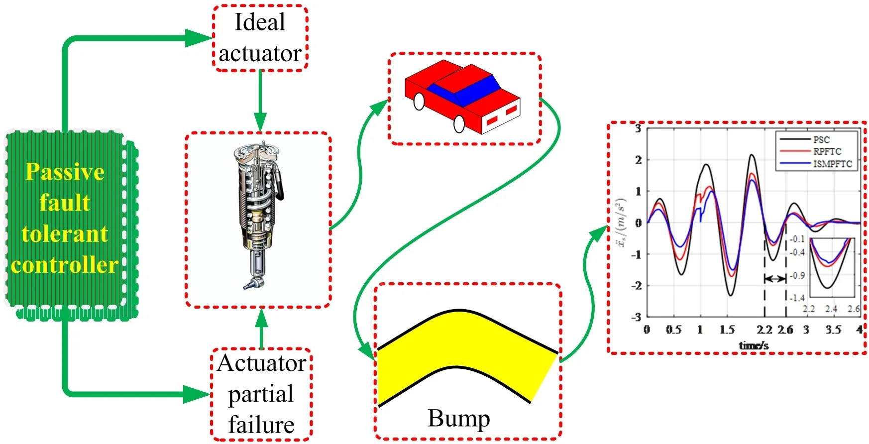
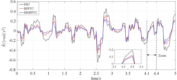
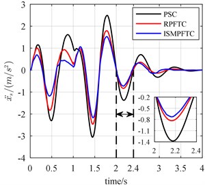
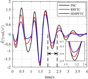
In the following work, let PSC represents passive suspension control, which is represented by a black solid line of the figure; RPFTC represents robust passive fault tolerant control based on $H_{2} / H_{\infty}$ approach, which is represented by a red solid line of the figure; ISMPFTC represents integral sliding mode passive fault tolerant control based on $H_{2} / H_{\infty}$ approach, which is represented by a blue solid line of the figure. In this section, the simulation results of passive fault tolerant control of a half-car model with actuator faults and model uncertainties are studied. All design parameters of the half-car model in Fig. 1 are listed in Table 1. The design parameters are derived from reference [7]. Road interference inputs to use filter white noise and bump response respectively. As to response of excitation of random road surface, in simulation, consider three cases, which are Case one, Case two, Case three; where Case one represents active suspension in good condition；Case two represents the percentage of disturbance of active suspension system parameters is –10 %; when $t =$ 2.5 s, the percentage of efficiency loss of the front and rear actuator all is 0.4; Case three represents the percentage of disturbance of active suspension system parameters is 10 %; when $t =$ 2.5 s, the percentage of efficiency loss of the front and rear actuator all is 0.8. Concerning bump response, in simulation, consider three cases too, which are Case one, Case two, Case three; but in each case, consider three different vehicle speeds, which are $v =$ 20 km/h, $v =$ 25 km/h, $v =$ 30 km/h; where Case one represents active suspension in good condition; the vehicle forwards velocity is 20 km/h, 25 km/h, 30 km/h respectively; Case two represents the percentage of disturbance of active suspension system parameters is –10 %; the vehicle for velocity is 20 km/h, 25 km/h, 30 km/h respectively; when $t =$ 1 s, the percentage of efficiency loss of the front and rear actuator all is 0.4; Case three represents the percentage of disturbance of active suspension system parameters is 10 %; the vehicle speed is 20 km/h, 25 km/h, 30 km/h respectively; when $t =$ 1 s, the percentage of efficiency loss of the front and rear actuator all is 0.8. The performances of vehicle suspension with passive suspension control, robust passive fault tolerant control based on $H_{2} / H_{\infty}$ approach, integral sliding mode passive fault tolerant control based on $H_{2} / H_{\infty}$ approach are compared in the time domain.

The vehicle is assumed to run linearly and the road condition for rear wheel is same as the front wheel, but with a time delay of $(a + b) / v$ . Using filtered white noise as the road inputs, the road input equations for the front and rear wheels are:

55

{\dot{x}}_{g i} = - 2 π f_{0} x_{g i} + 2 π \sqrt{G_{0} v} w_{i} (t), (i = 1,2),

where $f_{0}$ is low cut-off frequency, $f_{0} =$ 0.01 m^-1; $G_{0}$ is road roughness coefficient, $G_{0} =$ 5×10^-6 m³; $v =$ 20 m/s; $w_{i} (t)$ are white noise with zero mean and power spectral density of 1.

Consider the case of an isolated bump in a road surface, the bump road profile is described as follows:

56

x_{g i} = \{\begin{matrix} \frac{A_{0}}{2} (1 - (\cos \frac{2 π v}{L} t)), 0 \leq t \leq \frac{L}{v}, \\ 0, t > \frac{L}{v}, i = 1, 2, \end{matrix}

where $A_{0}$ and $L$ are the height and the length of the bump. Assume $A_{0} =$ 0.08 m, $L =$ 5 m, the vehicle forwards velocity is 20 km/h, 25 km/h, 30 km/h respectively.

The matrix $M_{0}$ , $J$ introduced in actuator fault model is $M_{0} = 0.5 ∙ e y e (2)$ , $J = e y e (2)$ , respectively. Constant matrices $H$ , $E_{1}$ , $E_{2}$ of appropriate dimensions in uncertainty model is:

E_{1} = [\begin{matrix} - 10.1961 0.6445 - 0.8497 0.0439 0 0 0.8497 - 0.0439 \\ 0.5273 - 14.4783 0.0439 - 0.9872 0 0 - 0.0439 0.9872 \\ 4.5000 0 0.3750 0 - 50 0 - 0.3750 0 \\ 0 6.1111 0 0.4167 0 - 55.5556 0 - 0.4167 \end{matrix}],

H = {[\begin{matrix} 0 & 0 & 1 & 0 & 0 & 0 & 0 & 0 \\ 0 & 0 & 0 & 1 & 0 & 0 & 0 & 0 \\ 0 & 0 & 1 & 0 & 0 & 0 & 20 & 0 \\ 0 & 0 & 1 & 0 & 0 & 0 & 0 & 16 \end{matrix}]}_{4 \times 8}^{T}, E_{2} = z e r o s (4.2) .

The obtained robust passive fault tolerant control law of the faulty suspension system based on $H_{2} / H_{\infty}$ approach is:

K_{f} = [\begin{matrix} - 1233.16 & 1567.53 & - 1289.19 & 10.50 & 4586.44 & 1175.35 & 203.60 & - 8.30 \\ - 897.95 & - 1735.59 & - 14.66 & - 1405.26 & - 1298.02 & 5894.45 & - 10.73 & - 319.45 \end{matrix}] .

As to integral sliding mode passive fault tolerant control, $ρ$ is a fixed scalar and the value is 150; the value of the small positive scalar $φ$ is chosen as $φ =$ 0.4, to eliminate chattering.

Table 1The vehicle system parameters for the half-car model

Description	Variable	Units	Value
Sprung mass	$m_{s}$	kg	690
Pitch moment of inertia	$I_{p}$	kg∙m	1222
Front tire stiffness	$K_{t 1}$	N/m	200000
Rear tire stiffness	$K_{t 2}$	N/m	200000
Front suspension stiffness	$K_{1}$	N/m	18000
Rear suspension stiffness	$K_{2}$	N/m	22000
Front unsprung mass	$m_{u 1}$	kg	40
Rear unsprung mass	$m_{u 2}$	kg	45
Front Sprung damping coefficient	$C_{s 1}$	N∙s/m	1000
Front Sprung damping coefficient	$C_{s 2}$	N∙s/m	1000
Actuator output threshold	$F_{m a x}$	N	1500
The maximum suspension working space	$S_{m a x}$	m	0.08
Distance of front axle to sprung mass c.g.	$a$	m	1.3
Distance of rear axle to sprung mass c.g.	$b$	m	1.5

5.1. Simulation results

5.1.1. Response of excitation of random road surface

Case one: active suspension in good condition, the simulation results are shown in Figs. 2-3.

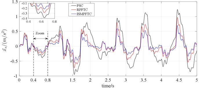
As for response to excitation of random road surface, in the first case, as is reflected in line charts 2-3 that the optimization effect are the integral sliding mode passive fault tolerant control based on $H_{2} / H_{\infty}$ approach is better than the robust passive fault tolerant control based on $H_{2} / H_{\infty}$ approach, and both of which are better than the passive suspension control.

Fig. 2Time-domain analysis of vertical acceleration of vehicle body

Case two: The percentage of disturbance of active suspension system parameters is –10 %; when $t =$ 2.5 s, the percentage of efficiency loss of the front and rear actuator all is 0.4, the simulation results are shown in the line charts 4-5.

Fig. 3Time-domain analysis of pitch acceleration

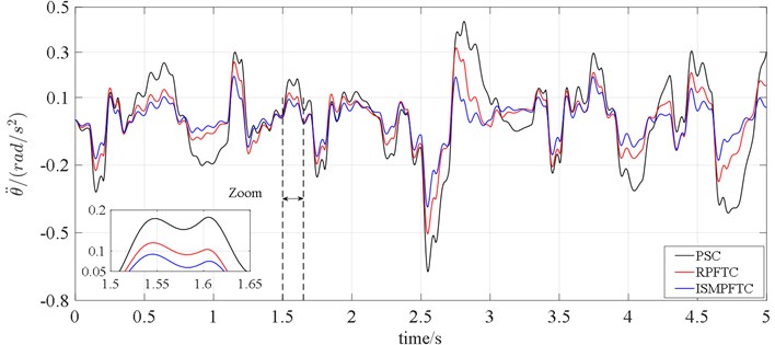
Fig. 4Time-domain analysis of vertical acceleration of vehicle body

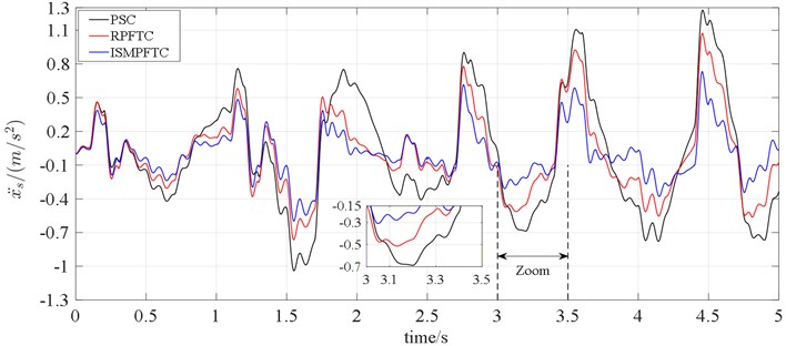
Fig. 5Time-domain analysis of pitch acceleration

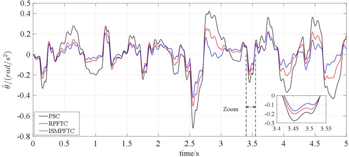
In Case two, when $t <$ 2.5 s, it can be seen from the line charts 4-5 that the control effect of the integral sliding mode passive fault tolerant control based on $H_{2} / H_{\infty}$ approach is the best, the robust passive fault tolerant control based on $H_{2} / H_{\infty}$ approach is the second best, the fault passive suspension control is the worst; when $t >$ 2.5 s, the order of the best optimization effects keeps the same.

Case three: The percentage of disturbance of active suspension system parameters is 10 %; when $t =$ 2.5 s, the percentage of efficiency loss of the front and rear actuator all is 0.8, the simulation results are shown in the line charts 6-7.

In Case three, when $t <$ 2.5 s, the line charts 6-7 illustrate that the optimization effect are the integral sliding mode passive fault tolerant control based on $H_{2} / H_{\infty}$ approach is better than the robust passive fault tolerant control based on $H_{2} / H_{\infty}$ approach, and both of which are better than the passive suspension control. When $t >$ 2.5 s, the control effect of the integral sliding mode passive fault tolerant control based on $H_{2} / H_{\infty}$ approach and the robust passive fault tolerant control based on $H_{2} / H_{\infty}$ approach is very close, but both of which are still slightly better than the passive suspension control.

Fig. 6Time-domain analysis of vertical acceleration of vehicle body

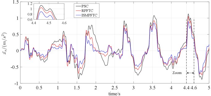
Fig. 7Time-domain analysis of pitch acceleration

5.1.2. Bump response

Case one: Active suspension in good condition; the vehicle forwards velocity is 20 km/h, 25 km/h, 30 km/h respectively; the simulation results are shown in Figs. 8-10.

Case two: The percentage of disturbance of active suspension system parameters is –10 %; the vehicle forwards velocity is 20 km/h, 25 km/h, 30 km/h respectively; when $t =$ 1 s, the percentage of efficiency loss of the front and rear actuator all is 0.4, the simulation results are shown in Figs. 11-13.

Case three: The percentage of disturbance of active suspension system parameters is 10 %; the vehicle forwards velocity is 20 km/h, 25 km/h, 30 km/h respectively; when $t =$ 1 s, the percentage of efficiency loss of the front and rear actuator all is 0.8, the simulation results are shown in Figs. 14-16.

Fig. 8The bump responses from body vertical acceleration, pitch angular acceleration (v= 20 km/h)

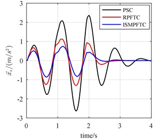
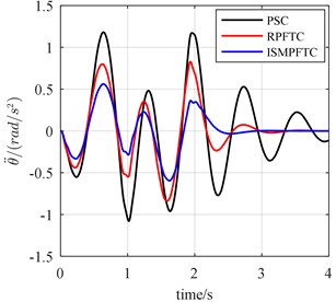
Fig. 9The bump responses from body vertical acceleration, pitch angular acceleration (v= 25 km/h)

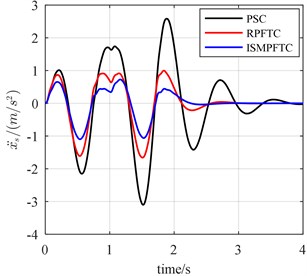
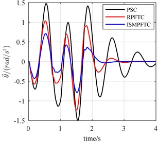
Fig. 10The bump responses from body vertical acceleration, pitch angular acceleration (v= 30 km/h)

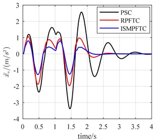
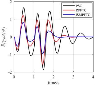
Fig. 11The bump responses from body vertical acceleration, pitch angular acceleration (v= 20 km/h)

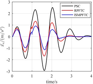
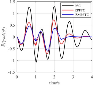
Fig. 12The bump responses from body vertical acceleration, pitch angular acceleration (v= 25 km/h)

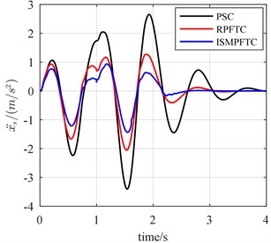
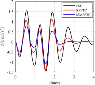
Fig. 13The bump responses from body vertical acceleration, pitch angular acceleration (v= 30 km/h)

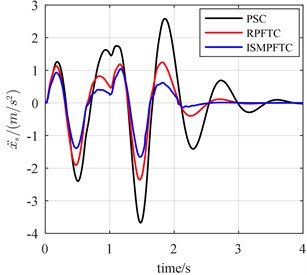
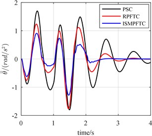
Fig. 14The bump responses from body vertical acceleration, pitch angular acceleration (v= 20 km/h)

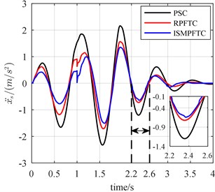
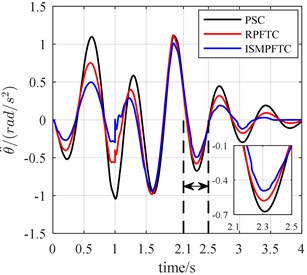
Fig. 15The bump responses from body vertical acceleration, pitch angular acceleration (v= 25 km/h)

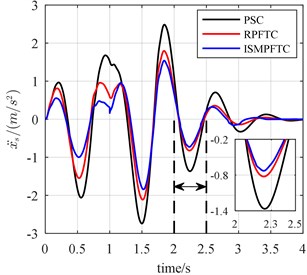
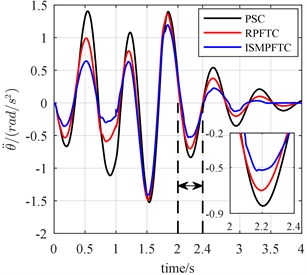
Fig. 16The bump responses from body vertical acceleration, pitch angular acceleration (v= 30 km/h)

Concerning bump response, in the first case, active suspension in good condition, the vehicle forwards velocity is 20 km/h, it can be seen from the line chart 8 that the optimization effect of the integral sliding mode passive fault tolerant control (ISMPFTC) based on $H_{2} / H_{\infty}$ approach is better than robust passive fault tolerant control (RPFTC) based on $H_{2} / H_{\infty}$ approach, and both of which are better than the passive suspension control. When the vehicle for velocity is 25 km/h, from Fig. 9, one can find that the order for optimization effects is all same as those shown in Fig. 8, which are that the control effect of the integral sliding mode passive fault tolerant control based on $H_{2} / H_{\infty}$ approach is the best, the robust passive fault tolerant control based on $H_{2} / H_{\infty}$ approach is the second best, the passive suspension control is the worst. As is displayed Fig. 10 that this is also true when the vehicle speed is 30 km/h.

In Case two, the percentage of disturbance of active suspension system parameters is 10 %. When the vehicle forwards velocity is 20 km/h, $t <$ 1 s, the front and rear actuators are fault free, as is revealed line chart 11 that the control effect of the integral sliding mode passive fault tolerant control (ISMPFTC) based on $H_{2} / H_{\infty}$ approach is better than robust passive fault tolerant control (RPFTC) based on $H_{2} / H_{\infty}$ approach, and both of which are better than the passive suspension control. When $t \geq$ 1 s, the percentage of efficiency loss of the front and rear actuator all is 0.4, from Fig. 11, it can be concluded that the order of the best optimization effects keeps the same. When the vehicle for velocity is 25 km/h, $t <$ 1 s, the front and rear actuators are trouble-free, as shown in the line chart 12 that the order for optimization effects is all same as those shown in Fig. 11. When $t \geq$ 1 s, the percentage of efficiency loss of the front and rear actuator all is 0.4, from Fig. 12, it can be seen that the order of the best optimization effects keeps the same, which are that the control effect of the integral sliding mode passive fault tolerant control based on $H_{2} / H_{\infty}$ approach is the best, the robust passive fault tolerant control based on $H_{2} / H_{\infty}$ approach is the second best, the passive suspension control is the worst. When the vehicle speed is 30 km/h, $t <$ 1 s, the front and rear actuators in good condition, the line chart 13 illustrates that the order of the best optimization effects is all same as those shown in Fig 12. When $t \geq$ 1 s, the percentage of efficiency loss of the front and rear actuator all is 0.4, as shown in the line chart 13 that the order of the best optimization effects keeps the same, which are that the optimization effect of the integral sliding mode passive fault tolerant control (ISMPFTC) based on $H_{2} / H_{\infty}$ approach is better than robust passive fault tolerant control (RPFTC) based on $H_{2} / H_{\infty}$ approach, and both of which are better than the passive suspension control.

In Case three, the percentage of disturbance of active suspension system parameters is 10 %. When the vehicle forwards velocity is 20 km/h, $t <$ 1 s, the front and rear actuators are fault free, as is displayed line chart 14 that the control effect of the integral sliding mode passive fault tolerant control based on $H_{2} / H_{\infty}$ approach is the best, the robust passive fault tolerant control based on $H_{2} / H_{\infty}$ approach is the second best, the passive suspension control is the worst. When $t \geq$ 1 s, the percentage of efficiency loss of the front and rear actuator all is 0.8, from Fig. 14, it can be seen that although the control effect of the integral sliding mode passive fault tolerant control based on $H_{2} / H_{\infty}$ approach and the robust passive fault tolerant control based on $H_{2} / H_{\infty}$ approach is very close, still slightly better than the passive suspension control. When the vehicle for velocity is 25 km/h, $t <$ 1 s, the front and rear actuators are trouble-free, as is reflected in line chart 15 that the order of optimization effects are all same as those shown in Fig. 14. When $t \geq$ 1 s, the percentage of efficiency loss of the front and rear actuator all is 0.8, from Fig. 15, as is revealed that the control effect of the integral sliding mode passive fault tolerant control based on $H_{2} / H_{\infty}$ approach and the robust passive fault tolerant control based on $H_{2} / H_{\infty}$ approach is very close, but still slightly better than the passive suspension control. When the vehicle speed is 30 km/h, $t <$ 1 s, the front and rear actuators in good condition, as shown in the line chart 16 that the order of the best optimization effects keeps the same. When $t \geq$ 1 s, the percentage of efficiency loss of the front and rear actuator all is 0.8, the line chart 16 illustrates that the control effect of the integral sliding mode passive fault tolerant control based on $H_{2} / H_{\infty}$ approach and the robust passive fault tolerant control based on $H_{2} / H_{\infty}$ approach is very close, but both of which are still slightly better than the passive suspension control.

Table 2RMS values of the performance indices for three failure modes

RMS	Case one
Parameter	${\ddot{x}}_{s}$	$\ddot{θ}$	${\ddot{x}}_{s}$	$\ddot{θ}$	${\ddot{x}}_{s}$	$\ddot{θ}$	${\ddot{x}}_{s}$	$\ddot{θ}$
PSC	0.4852	0.1931	1.2473	0.6163	1.3466	0.7614	1.3668	0.8321
RPFTC	0.3005	0.1195	0.6735	0.4106	0.7464	0.5201	0.7939	0.5907
ISMPFTC	0.2008	0.0797	0.4243	0.2633	0.4762	0.3163	0.5145	0.3568
Road type	Random road		$v =$ 20 km/h		$v =$ 25 km/h		$v =$ 30 km/h
Road type	Random road		Bump road
RMS	Case two
Parameter	${\ddot{x}}_{s}$	$\ddot{θ}$	${\ddot{x}}_{s}$	$\ddot{θ}$	${\ddot{x}}_{s}$	$\ddot{θ}$	${\ddot{x}}_{s}$	$\ddot{θ}$
PSC	0.5074	0.2063	1.3642	0.6604	1.4435	0.7833	1.4352	0.8300
RPFTC	0.3338	0.1240	0.7754	0.4605	0.8366	0.5688	0.8682	0.6234
ISMPFTC	0.2201	0.0876	0.5099	0.3241	0.5641	0.3883	0.6006	0.4252
Road type	Random road		$v =$ 20 km/h		$v =$ 25 km/h		$v =$ 30 km/h
Road type	Random road		Bump road
RMS	Case three
Parameter	${\ddot{x}}_{s}$	$\ddot{θ}$	${\ddot{x}}_{s}$	$\ddot{θ}$	${\ddot{x}}_{s}$	$\ddot{θ}$	${\ddot{x}}_{s}$	$\ddot{θ}$
PSC	0.4549	0.1855	1.1114	0.5625	1.2049	0.7192	1.2016	0.7798
RPFTC	0.3607	0.1267	0.7552	0.4490	0.8423	0.5876	0.8836	0.6509
ISMPFTC	0.2923	0.1051	0.5935	0.3745	0.6610	0.4876	0.7055	0.5390
Road type	Random road		$v =$ 20 km/h		$v =$ 25 km/h		$v =$ 30 km/h
Road type	Random road		Bump road

RMS values of the performance indices of the half-car model with three failure modes are listed in Table 2 for quantifying and comparing the effects of these three control methods in different situations. It can be reached from Figs. 8-16 and Table 2 that at different vehicle speeds and failure modes, the optimization effect of the integral sliding mode passive fault tolerant control (ISMPFTC) based on $H_{2} / H_{\infty}$ approach is better than robust passive fault tolerant control (RPFTC) based on $H_{2} / H_{\infty}$ approach, and both of which are better than the passive suspension control. The proposed control methods are robust to the actuator faults and model uncertainties. The above simulation analysis show: whether the active suspension system is in good condition or malfunction in actuators and model uncertainties, both the integral sliding mode passive fault tolerant control and the robust passive fault tolerant control can improve the ride comfort of the suspension system to a certain extent.

6. Conclusions

In this study, the partial fault of actuators, time-domain hard constraints and model uncertainties of the suspension system are considered. A robust passive fault-tolerant control (RPFTC) strategy and an integral sliding mode passive fault tolerant control (ISMPFTC) strategy are investigated; two passive fault-tolerant control strategies based on $H_{2} / H_{\infty}$ approach have been applied to an active suspension system respectively. Road interference inputs to use filter white noise and bump response respectively. As to response of excitation of random road surface, in simulation, consider three cases. Concerning bump response, in simulation, consider three cases too, but in each case, consider three different vehicle speeds, which are $v =$ 20 km/h, $v =$ 25 km/h, $v =$ 30 km/h. Finally, an analysis of the simulation results is given to verify the feasibility and effectiveness of the proposed two control strategies is the main contributions of this work. The research we have done suggests that the two passive fault-tolerant control strategies are robust to the actuator faults and model uncertainties, and can guarantee the stability of the vehicle active suspension system, improve the ride comfort of the vehicle simultaneously to a certain degree.

References

Chen W. W., Wang Q. D., Xiao H. S., Zhang L. F. Integrated Vehicle Dynamics and Control. Wiley, 2016.

Publisher
Isermann R. Mechatronic Systems: Fundamentals. Springer-Verlag, 2005.

Search CrossRef
Tseng H. E., Hrovat D. State of the art survey: active and semi-active suspension control. Vehicle System Dynamics, Vol. 53, Issue 7, 2015, p. 1034-1062.

Publisher
Gillespie D T. Fundamentals of Vehicle Dynamics. Society of Automotive Engineers, 1992.

Publisher
Rajamani R. Vehicle Dynamics and Control. Springer Science and Business Media, 2011.

Publisher
Cao D. P., Song X. B., Ahmadian M. Editors’ perspectives: road vehicle suspension design, dynamics, and control. Vehicle System Dynamics, Vol. 49, Issues 1-2, 2011, p. 3-28.

Publisher
Liu H. H., Gao H., Li P. Handbook of Vehicle Suspension Control Systems. United Kingdom, 2013.

Search CrossRef
Chen H., Guo K. An LMI approach to multi-objective RMS gain for active suspensions. Proceedings of the American Control Conference, Vol. 4, 2001, p. 2646-2651.

Search CrossRef
Chen H., Guo K. Constrained H∞ control of active suspensions: an LMI approach. IEEE Transactions on Control Systems Technology, Vol. 13, Issue 3, 2005, p. 412-421.

Publisher
Chen G. D., Yang Yu M. Y. L. Mixed H2/H∞ optimal guaranteed cost control of uncertain linear systems. Journal of Systems Science and Information, Vol. 2, Issue 3, 2004, p. 409-416.

Search CrossRef
Guo L. X., Zhang L. P. Robust H∞ control of active vehicle suspension under non-stationary running. Journal of Sound and Vibration, Vol. 331, Issue 26, 2012, p. 5824-5837.

Publisher
Soliman H. M., Bajabaa N. S. Robust guaranteed-cost control with regional pole placement of active suspensions. Journal of Vibration and Control, Vol. 19, Issue 8, 2013, p. 1170-1186.

Publisher
Bharalil J., Buragohain M. Design and performance analysis of fuzzy LQR; fuzzy PID and LQR controller for active suspension system using 3 degree of freedom quarter car model. IEEE International Conference on Power Electronics, Intelligent Control and Energy Systems, Delhi, India, 2016.

Publisher
Bououden S., Chadli M., Zhang L. X., Yang T. Constrained model predictive control for time varying delay systems: application to an active car suspension. International Journal of Control, Automation, and Systems, Vol. 14, Issue 1, 2016, p. 51-58.

Publisher
Blanke M., Kinnaert M., Lunze D. I. J. Introduction to diagnosis and fault-tolerant control. Diagnosis and Fault-Tolerant Control, Vol. 49, Issue 6, 2003, p. 1-32.

Publisher
Alwi H., Edwards C., Tan C. P. Fault Detection and Fault-Tolerant Control Using Sliding Modes. Springer London, 2011.

Publisher
Patton R. J. Fault-tolerant control systems: the 1997 situation. IFAC Symposium on Fault Detection Supervision and Safety for Technical Processes, 1997.

Publisher
Zhang Y., Jiang J. Bibliographical review on re-configurable fault-tolerant control systems. Annual Reviews in Control, Vol. 32, Issue 2, 2008, p. 229-252.

Publisher
Benosman M. Passive Fault Tolerant Control. INTECH Open Access Publisher, 2011.

Publisher
Yang X. Z., Hong G. Robust adaptive fault-tolerant compensation control with actuator failures and bounded disturbances. Acta Automatica Sinica, Vol. 35, Issue 3, 2009, p. 305-309.

Publisher
Gholami M. Passive fault tolerant control of piecewise affine systems based on H infinity synthesis. IFAC Proceedings, Vol. 44, Issue 1, 2011, p. 3084-3089.

Publisher
Jiang J. Fault-tolerant Control Systems-An Introductory Overview. Acta Automatica Sinica, Vol. 31, Issue 1, 2005, p. 161-174.

Search CrossRef
Li H., Gao H., Liu H., Li M. Fault-tolerant H∞ control for active suspension vehicle systems with actuator faults. Proceedings of the Institution of Mechanical Engineers, Part I: Journal of Systems and Control Engineering, Vol. 226, Issue 3, 2012, p. 348-363.

Publisher
Sun W. C., Pan H. H., Yu J. Y., Gao H. J. Reliability control for uncertain half-car active suspension systems with possible actuator faults. IET Control Theory and Applications, Vol. 8, Issue 9, 2014, p. 746-754.

Publisher
Wang R., Jing H., Karimi H. R., Chen N. Robust fault-tolerant H∞ control of active suspension systems with finite-frequency constraint. Mechanical Systems and Signal Processing, Vol. 62, 2015, p. 341-355.

Publisher
Liu B., Saif M., Fan H. Adaptive fault tolerant control of a half-car active suspension systems subject to random actuator failures. IEEE/ASME Transactions on Mechatronics, Vol. 21, Issue 6, 2016, p. 2847-2857.

Publisher
Hamayun M. T., Edwards C., Alwi H. Fault Tolerant Control Schemes Using Integral Sliding Modes. Springer International Publishing, 2016.

Publisher
Sam Y. M., Osman J. H., Ghani M. R. A. A class of proportional-integral sliding mode control with application to active suspension system. Systems and Control Letters, Vol. 51, Issue 3, 2004, p. 217-223.

Publisher
Chamseddine A., Noura H., Ouladsine M. Sensor fault-tolerant control for active suspension using sliding mode techniques. Workshop on Networked Control Systems and Fault-Tolerant Control, 2005.

Publisher
Dong Yu Guan X. M. Z. Adaptive sliding mode fault-tolerant control for semi-active suspension using magnetorheological dampers. Journal of Intelligent Material Systems and Structures, Vol. 22, Issue 15, 2011, p. 1653-1660.

Publisher
Moradi M., Fekih A. Adaptive PID-sliding-mode fault-tolerant control approach for vehicle suspension systems subject to actuator faults. IEEE Transactions on Vehicular Technology, Vol. 63, Issue 3, 2014, p. 1041-1054.

Publisher
Moradi M., Fekih A. A stability guaranteed robust fault tolerant control design for vehicle suspension systems subject to actuator faults and disturbances. IEEE Transactions on Control Systems Technology, Vol. 23, Issue 3, 2015, p. 1164-1171.

Publisher

Cited by

RBF-Based Fractional-Order SMC Fault-Tolerant Controller for a Nonlinear Active Suspension

Weipeng Zhao | Liang Gu

(2024)

Adaptive fault-tolerant control of high-speed maglev train suspension system with partial actuator failure: design and experiments

Yougang Sun | Fengxing Li | Guobin Lin | Junqi Xu | Zhenyu He

(2023)

A Robust Control for a Controllable Suspension System with an Input Time Delay

Honglin Zhu | Weiping Ding | Mingliang Yang | Tianshi Jin

(2023)

Research on robust fault-tolerant control of the controllable suspension based on knowledge-data fusion driven

Honglin Zhu | Weiping Ding | Mingliang Yang | Yudong Wu | Tong Du

(2023)

H 2 Performance Analysis of Tractors Traveling on Rough Terrain

Shinsaku Izumi | Riku Hayashida | Xin Xin

(2022)

Longitudinal–vertical comprehensive control for four-wheel drive pure electric vehicle considering energy recovery and ride comfort

Junjiang Zhang | Yang Yang | Minghui Hu | Zhong Yang | Chunyun Fu

(2021)

2020 39th Chinese Control Conference (CCC)

Yun Zhang | Ming Yu | Bing Wang | Chenyu Xiao

(2020)

A novel fault tolerant control approach based on backstepping controller for a five phase induction motor drive: Experimental investigation

Mahmoud A. Mossa | Hamdi Echeikh

(2020)

About this article

Received

20 February 2017

Accepted

12 December 2017

Published

30 June 2018

SUBJECTS

Vibration in transportation engineering

DOI

https://doi.org/10.21595/jve.2017.18264

Keywords

active suspension

H2/H∞ control

parameter uncertainties

actuator faults

RPFTC

ISMPFTC

Acknowledgements

This work was supported by the Excellent Talents Project for the Second Level in the Education Department, Liaoning Province, China (No. LJQ2014065); Soft Science Research Plan Project, Science and Technology Department, Liaoning Province, China (No. JP2016017).

This is an open access article distributed under the Creative Commons Attribution License, which permits unrestricted use, distribution, and reproduction in any medium, provided the original work is properly cited.

Previous article in issue Previous Next article in issue Next

Research article

2019 08 15

Multi-objective optimization of active suspension predictive control based on improved PSO algorithm

Qiang Zhao, Baoquan Zhu

Research article

2018 11 15

Active control of a nonlinear suspension with output constraints and variable-adaptive-law control

Jun Yao, Jin Qiu Zhang, Ming Mei Zhao, Xin Li

Research article

2018 02 15

Adaptive Neuro Fuzzy Inference System control of active suspension system with actuator dynamics

P. Senthil Kumar, K. Sivakumar, R. Kanagarajan, S. Kuberan

Research article

2017 03 31

Discrete approximate optimal vibration control for nonlinear vehicle active suspension

Shi-Yuan Han, Xiao-Fang Zhong, Yue-Hui Chen, Gong-You Tang

L. P. Zhang and D. L. Gong, “Passive fault-tolerant control for vehicle active suspension system based on H2/H∞ approach,” Journal of Vibroengineering, Vol. 20, No. 4, pp. 1828–1849, Jun. 2018, https://doi.org/10.21595/jve.2017.18264

Copy Extrica

Copied to clipboard!

TY  - JOUR
DO  - 10.21595/jve.2017.18264
UR  - https://doi.org/10.21595/jve.2017.18264
TI  - Passive fault-tolerant control for vehicle active suspension system based on H2/H∞ approach
T2  - Journal of Vibroengineering
AU  - Zhang, Li Ping
AU  - Gong, Dong Liang
PY  - 2018
DA  - 2018/06/30
PB  - JVE International Ltd.
SP  - 1828-1849
IS  - 4
VL  - 20
SN  - 1392-8716
SN  - 2538-8460
ER  - 

Copy Ris

Copied to clipboard!

@article{Zhang_2018,
	doi = {10.21595/jve.2017.18264},
	url = {https://doi.org/10.21595/jve.2017.18264},
	year = 2018,
	month = {jun},
	publisher = {{JVE} International Ltd.},
	volume = {20},
	number = {4},
	pages = {1828--1849},
	author = {Li Ping Zhang and Dong Liang Gong},
	title = {Passive fault-tolerant control for vehicle active suspension system based on H2/H$\infty$ approach},
	journal = {Journal of Vibroengineering}
}

Copy Bibtex

Copied to clipboard!

[1]L. P. Zhang and D. L. Gong, “Passive fault-tolerant control for vehicle active suspension system based on H2/H∞ approach,” Journal of Vibroengineering, vol. 20, no. 4, pp. 1828–1849, Jun. 2018, doi: 10.21595/jve.2017.18264.

Copy IEEE

Copied to clipboard!

Zhang, Li Ping, and Dong Liang Gong. “Passive Fault-Tolerant Control for Vehicle Active Suspension System Based on H2/H∞ Approach.” Journal of Vibroengineering 20, no. 4 (June 30, 2018): 1828–49. https://doi.org/10.21595/jve.2017.18264.

Copy Chicago

Copied to clipboard!

Passive fault-tolerant control for vehicle active suspension system based on H2/H∞ approach

Abstract

Highlights

1. Introduction

2. Half-car model

3. Modeling of faulty systems

3.1. Actuator fault model

3.2. Uncertainty model

3.3. The fault suspension model

4. Passive fault-tolerant controller design

4.1. Robust passive fault-tolerant controller design based on H2/H∞ approach

4.2. Integral sliding mode fault-tolerant controller design based on H2/H∞ approach

4.2.1. Integral switching surface

4.2.2. Integral sliding mode control laws

4.2.3. The reachability condition

5. Illustrative examples

5.1. Simulation results

5.1.1. Response of excitation of random road surface

5.1.2. Bump response

6. Conclusions

References

Cited by

About this article

Related Articles

4.1. Robust passive fault-tolerant controller design based on $H_{2} / H_{\infty}$ approach

4.2. Integral sliding mode fault-tolerant controller design based on $H_{2} / H_{\infty}$ approach