Abstract
This paper studies the discrete actuator-fault-tolerant control problem for a vehicle active suspension system under persistent road disturbances. The discrete model of vehicle active suspension with actuator faults is formulated firstly, in which the actuator faults are described as the output of an exogenous system with unknown initial values. By designed a fault diagnoser, the optimal actuator-fault-tolerant controller is derived from the discrete Riccati equation and Stein equations, respectively. Simulation results illustrate that the ride comfort, road holding ability, and suspension deflection can be reduced significantly and the reliability of the vehicle active suspension can be improved.
1. Introduction
As an effective component for vehicle active safety technology, vehicle active suspension systems can meet the various requirements of performance criterions, such as road holding ability, ride comfort, and suspension deflection. Compared with the traditional passive and semi-passive suspensions, vehicle active suspension systems are able to store, dissipate and generate energy [1, 2]. Then, the stability can be guaranteed and the better control performance can be achieved by using the novel control strategies and advanced actuators. Many advanced control schemes have been proposed for vehicle active suspension in recent decades. For instance, a control scheme was designed to trade off among multi-objective requirements for uncertain nonlinear active suspension in [3]; an enhance adaptive self-organizing fuzzy sliding-mode controller was proposed for active suspension systems in [4]; [5] designed a discrete feedback and feedforward optimal vibration controller for vehicle active suspension with actuator time delay. Also, the art survey about active and semi-active suspension control was given in [6].
The development of actuator-fault-tolerant controller is beneficial to improve the reliability of the suspension systems. Due to the actuator faults, the generated actuator force maybe not researched the expected value. Then, the serious degradation of control performance will generate, even the suspension system becomes instability. To eliminate the influence from actuator faults and ensure the safety of the suspension systems, many researchers have paid more attention to fault-tolerant control problem. For example, an adaptive sliding fault tolerant controller was proposed for nonlinear uncertain active suspension system in [7]; considering the actuator faults, an adaptive PID-Sliding-Mode fault tolerant control scheme was developed in [8]; a reliable fuzzy controller was proposed for active suspension systems with actuator delay and fault in [9]. The above active control schemes are capable of reducing the vibration of vehicle active suspension subject to road disturbances and actuator faults. However, the rarely digital fault-tolerant control problem is considered for vehicle active suspension under computer control system. Actually, with advantages of low-cost components and conveniences of digital systems, the digital control becomes the tendency of the development of the vehicle active suspension [10]. Recently, the various methods have been applied to the actuator-fault-tolerant control problem for computer control systems, such as control [11], stochastic control [12], and observer-based control [13]. However, there are few results about the discrete actuator-fault-tolerant controller design for vehicle active suspension in the sense of the optimal perspective.
The above considerations motivate our research in the present work. Taken the actuator faults into consideration, the discrete model of the vehicle active suspension is developed, in which the persistent road disturbances and actuator faults are described as the outputs of the designed exogenous systems with unknown initial values. Then, an optimal discrete quadratic optimal actuator-fault-tolerant controller is proposed to offset the vibration of vehicle body caused by the road disturbances and overcome the unsafely caused by the actuator faults. Meanwhile, a fault observer is designed to diagnose the actuator faults so that the physically unrealizable problem of the proposed controller is solved. Simulation results are shown that the control performance and reliability of the vehicle active suspension can be improved by using the proposed controller.
The paper is organized as follows. The discrete optimal fault-tolerant control problem of the vehicle active suspension is formulated in Section 2. Section 3 is devoted to present the main results, where an actuator-fault-observer-based discrete optimal fault-tolerant controller is proposed. Section 4 provides some simulation results to illustrate the effectiveness of the developed approaches. Finally, Section 5 gives the conclusion of this paper.
2. Problem formulation
2.1. Discrete suspension modeling with actuator faults
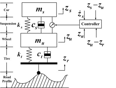
As shown in Fig. 1, a simple vehicle active suspension with actuator faults is considered in this paper. The global dynamic equations of the vehicle active suspension can be described as:
where and represent the sprung mass and unsprung mass, respectively; and are the compressibility and damping of the pneumatic tire; and stand for the stiffness and damping of the passive suspension system, respectively. and denote the displacements of the sprung and unsprung masses. is the control force of the vehicle active suspension, and represent the road disturbances and the actuator fault acting on the vehicle active suspension, respectively.
Define the following state variables:
where is the suspension deflection, denotes the tire deflection, is the sprung mass velocity, and denotes the unsprung mass velocity.
Let , the state-space model of the vehicle active suspension (1) subject to the actuator faults can be formulated as:
where:
Fig. 1Simple vehicle active suspension
Remark 1: The sprung mass acceleration , the suspension deflection , and the tire deflection are viewed as the main performance criteria, which directly relate to the ride comfort, the road holding ability, and driving safety ability directly. Hence, we design the controlled output as the second formula of (3).
The following exogenous system is introduced to describe the dynamic characteristics of the actuator fault :
where is the state vector of the actuator faults, and are constant matrices with appropriate dimensions. The actuator fault occurs at , in which the initial fault time and the initial fault state are unknown.
Let denotes the sampling period, the discrete model of vehicle active suspension system (3) can be expressed as:
where , , , and .
The discrete representation of the actuator fault Eq. (5) can be obtained:
where .
Remark 2: Various kinds of the actuator faults can be described as Eq. (7) with known dynamic characteristics, and unknown magnitudes and phases, such as periodic faults, sinusoidal faults, and other actuator faults in the discrete form.
Assumption 1: The pair is controllable and the pair is observable.
Assumption 2: The pair is completely observable, and all the eigenvalues of satisfy .
2.2. Road disturbances
As stated in [6], the road disturbances can be derived from a random process with ground displacement power spectral density (PSD):
where denotes a spatial frequency, is a reference frequency. The value of denotes the measurement for the road roughness, where and are the roughness constants.
The road displacement input from road irregularities in Eq. (1) can be written as the following series:
where, is the length of the road segment, are the random variables, is the initial with time frequency internal, and is used to restrict the frequency range of vehicle body. Then, the road disturbance in Eq. (3) can be described as:
Define the following state space vectors:
Then the state space representation of road disturbance can be obtained:
where:
Remark 3: Because the , the pair is observable.
Under the sampling period , the discrete state space model of road disturbance Eq. (12) can be described as:
where . It is assumed that the eigenvalues of satisfy .
As mentioned in Remark 1, in order to improve the control performance of vehicle active suspension, the average quadratic performance index is chosen as:
where is a positive semi-definite matrix, is a constant.
Our aim is to design a discrete fault observer to diagnose the actuator faults of vehicle active suspension, thereby to design a discrete optimal actuator-fault-tolerant control law for system Eq. (6) subject to actuator faults Eq. (7) and persistent road disturbances Eq. (14) to minimum the average quadratic performance index Eq. (15).
In order to obtain the discrete optimal actuator-fault-tolerant controller, a lemma is introduced first [14].
Lemma 1: Let , , , and . The matrix equation:
has a unique solution if and only if:
where are eigenvalues of matrix.
3. Design of discrete optimal fault-tolerant controller via an actuator fault observer
In this section, we propose a discrete optimal fault-tolerant controller first and prove the existence and uniqueness of the designed controller. Then, a discrete fault observer is designed to solve the physically unrealizable problem caused by the status vector of actuator faults.
3.1. Design of discrete optimal actuator-fault-tolerant control scheme
The designed discrete optimal actuator-fault-tolerant control law will be described in Theorem 1. In order to state the Theorem 1 conveniently, the following matrices are defined:
Theorem 1: Consider the discrete optimal actuator-fault-tolerant control problem for vehicle active suspension system Eq. (6) under actuator faults Eq. (7) and road disturbances Eq. (14) with respect to quadratic performance index Eq. (15), under Assumptions Eqs. (1) and (2), there exists a unique discrete optimal actuator-fault-tolerant control law in the form as:
where is a positive semi-definite matrix solution to the discrete Riccati equation:
with , and the matrices and are the unique solutions of the following Stein equations:
Proof: Based on the classical optimal theory, the optimal actuator-fault-tolerant control law for system Eq. (6) with respect to the performance index Eq. (15) can be described as:
where satisfies the following two-point boundary value problem:
In order to solve Eq. (23), we introduce the following equation:
From the second formula in Eq. (23), can be described as:
Then, substituting Eq. (25) into Eq. (22), we obtain the discrete optimal actuator-fault-tolerant control law Eq. (19).
Substituting Eq. (24) into the first formula in Eq. (23), noting Eq. (13) and Eq. (14), one yields:
Based on Eqs. (23), (25) and (26), one gets:
Comparing the parameters of Eqs. (24) and (27), we obtain discrete Riccati matrix Eq. (20) and Stein matrices Eq. (21).
The existence and uniqueness of the matrices , and will be proved in the following.
From Assumption 1 and classic optimal control theory, is the positive semi-definite matrix solution of discrete Riccati Eq. (20). Based on the linear regulator theory, noting Eqs. (23) and (25), one gets:
Then, we obtain:
Therefore, the matrices and are the unique solutions of the Stein Eq. (21). Therefore, the proposed controller Eq. (19) is uniqueness. The proof is completed.
3.2. Design of an actuator fault observer
The discrete optimal actuator-fault-tolerant controller Eq. (19) is physically unrealizable due to the vector items and . In order to make the proposed controller more practical, an actuator fault observer will be designed in this subsection.
Introduce a discrete actuator fault observer as:
where is the state of the fault observer, is the fault diagnosis value of the actuator fault , serves as a gain weighting matrix to be determined, is the initial value of the actuator fault observer.
Denote the fault diagnosis error as:
where is the initial error.
From Eqs. (7) and (31), one yields:
Due to the fact from Assumption 2 that the pair is completely observable, the diagnosis gain matrix can be designed based on a set of given poles such that:
which means that the actuator faults can be diagnosed in vehicle active suspension.
Then, based on the diagnosis value of the actuator faults, the proposed discrete actuator-fault-tolerant controller Eq. (19) can be rewritten as:
where is obtained from the actuator fault observer Eq. (30).
Remark 4: Due to the fact that the diagnosis values of the actuator faults are used in the design of control law Eq. (31). We can choose the observer gain matrix such that all the eigenvalues of the matrix are assigned to the expected positions of the unit circle of the plane. In general, we always choose to make the observer converge quicker than the original controlled system.
Then, the system structure of vehicle active suspension is shown as Fig. 2.
4. Simulation results
In this section, we will apply the proposed optimal actuator-fault-tolerant control law to a vehicle active suspension. The parameters of a vehicle active suspension are shown in Table 1.
Fig. 2The system structure of vehicle active suspension
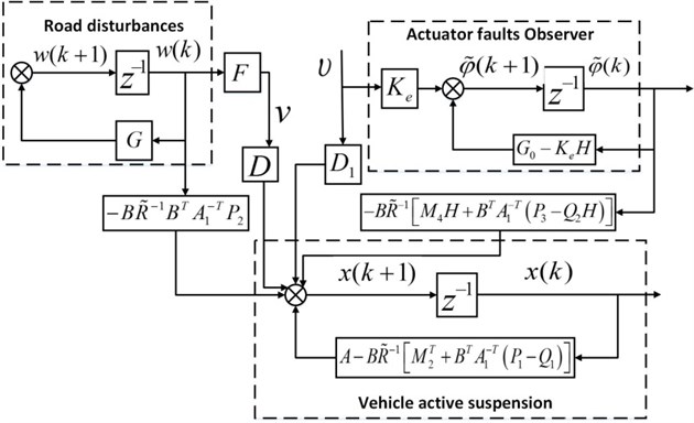
Table 1The parameters of a vehicle active suspension
Name | Variable | Value | Unit |
Sprung mass | N | ||
Unsprung mass | N | ||
Damping of the passive suspension system | Ns/m | ||
Stiffness of the passive suspension system | N/m | ||
Compressibility of the pneumatic tire | N/m | ||
Damping of the pneumatic tire | Ns/m |
Then, defining the sampling period 0.08 s, the matrices in Eq. (3) can be obtained:
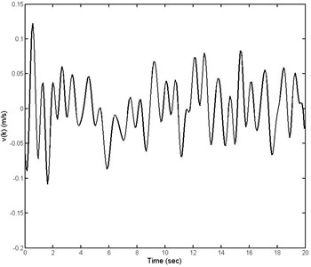
The road displacement input is generated from a ground displacement PSD (8), where 256×10-6 m3 with 2 and 1.5. Under 20 m/s and 400 m, the road disturbances acting on the vehicle active suspension can be computed, which is depicted in Fig. 3.
Two types of actuator faults are considered in this section, which include attenuation type and oscillation type. Assume that the actuator fault occurs at 4 s, and the initial value of the actuator fault .
For attenuation type of actuator fault, the matrices and is given by:
Designing the poles of the actuator fault observer as 0.48±0.5i, the gain weighting matrix is obtained as .
For oscillation type of actuator fault, the matrices and are given as follows:
Fig. 3The curve of random road disturbances
Designing the poles of the actuator fault observer as 0.3±0.19i, the gain weighting matrix is obtained as . The comparison results between real actuator faults and the actuator fault observer are shown in Fig. 4. It can be seen clearly that the actuator fault , can be diagnosed in 4s exactly by using the designed actuator fault observer Eq. (30).
Setting the initial status , the weight matrices and 1, by solving the discrete Riccati Eq. (20) and Stein Eqs. (21), respectively, the feedforward and feedback optimal actuator-fault-tolerant controller (FFOAFTC) under two types of actuator faults Eqs. (36) and (37) can be obtained. Meanwhile, the feedback optimal actuator-fault-tolerant controller (FOAFTC) without feedforward item of actuator faults is used to compare with the proposed FFOAFTC, which is described as:
The curves of FFOAFTC and FOAFTC under attenuation type and oscillation type of actuator fault are shown in Fig. 5.
When the optimal FFOAFTC acts on the vehicle active suspension, the response curves of the sprung mass acceleration (SMA), sprung deflection (SD), and tire deflection (TD) are shown in Figs. 6-8, respectively, in which the results are compared with ones of FOAFTC and open-loop (OL) systems. From these figures, one can be seen that during the actuator faults period, the values of SMA, SD, and TD converge to smaller values by using the FFOAFTC.
In order to show the ability of controller to reduce the vibration amplitude, the frequency spectrums of SMA, SD, and TD in presence of both actuator faults are shown in Figs. 9-11 compared with FOAFTC and uncontrolled ones.
Meanwhile, in order to show the effectiveness of the proposed FFOAFTC clearly, the peak values and root-mean square (RMS) values of SMA, SD, and TD are compared with FOAFTC and uncontrolled ones in Table 2. For example, under the attenuation type of actuator fault, the peak value of SMA is reduced about 23.3 % compared to the OL one by using the proposed FFOAFTC, the RMS value of the SMC is reduced about 70.4 %, the RMS of sprung deflection is reduced about 69.3 %, and the RMS of tire deflection is reduced about 60.4 % less than that of OL system.
Fig. 4The comparison between real actuator fault and actuator fault observer
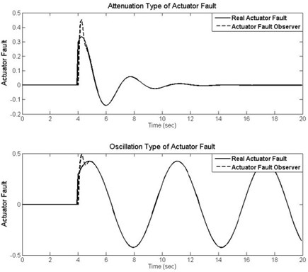
Fig. 5The curves of control law for attenuation type and oscillation type of actuator fault
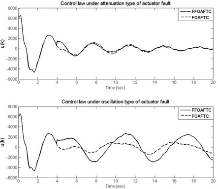
Fig. 6The curves of SMA under different actuator fault types
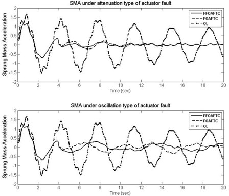
Fig. 7The curves of SD under different actuator fault types
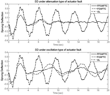
Fig. 8The curves of TD under different actuator fault types
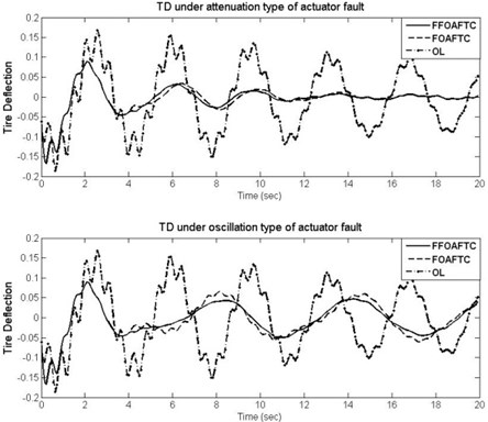
Fig. 9The frequency spectrums of SMA under different actuator fault types
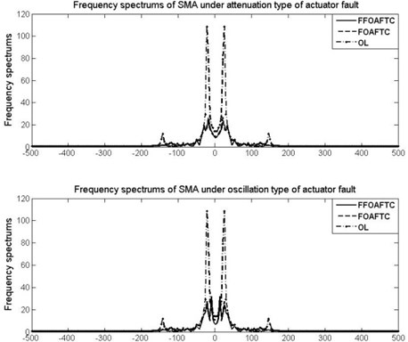
Fig. 10The frequency spectrums of SD under different actuator fault types
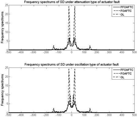
Fig. 11The frequency spectrums of TD under different actuator fault types
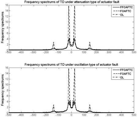
Table 2Peak and RMS values of performance criteria and controller under different actuator fault
Name | Fault | SMA | SD | TD | (103) | |
Peak values | OL | \ | 1.691 | 0.3661 | 0.1894 | \ |
FFOAFTC | Attenuation | 1.297 (–23.3%) | 0.263 (–28.2%) | 0.161 (–15.0%) | 6.4831 | |
Oscillation | 1.297 (–23.3%) | 0.263 (–28.2%) | 0.161 (–15.0%) | 6.4831 | ||
FOAFTC | Attenuation | 1.297 (–23.3%) | 0.263 (–28.2%) | 0.161 (–15.0%) | 6.4831 | |
Oscillation | 1.297 (–23.3%) | 0.263 (–28.2%) | 0.161 (–15.0%) | 6.4831 | ||
RMS values | OL | \ | 1.025 | 0.228 | 0.101 | \ |
FFOAFTC | Attenuation | 0.303 (–70.4%) | 0.070 (–69.3%) | 0.040 (–60.4%) | 1.7342 | |
Oscillation | 0.311 (–69.7%) | 0.072 (–68.4%) | 0.040 (–60.4%) | 1.7495 | ||
FOAFTC | Attenuation | 0.324 (–68.4%) | 0.075 (–67.1%) | 0.049 (51.5%) | 2.3480 | |
Oscillation | 0.326 (–68.2%) | 0.102 (–55.3%) | 0.051 (49.5%) | 1.7892 | ||
From Table 2 and Figs. 4-11, it can be found that the designed observer can diagnose the actuator fault exactly, and the proposed optimal actuator-fault-tolerant controller can effectively compensate the actuator fault and offset the vehicle body’s vibration caused by road disturbances. The control performance of vehicle active suspension is improved significantly.
5. Conclusions
This paper has researched the problem of discrete actuator-fault-tolerant control problem for a class of vehicle active suspension. Different from the previous approaches, with regarded the actuator faults as an output of exosystem with unknown initial value and occurred time, the discrete model of vehicle active suspension with actuator faults was established first. Furthermore, an optimal actuator-fault-tolerant control scheme was devised from discrete Riccati equation and Stein equations. What’s more, an actuator fault observer was designed to make the control scheme physical realizability. Then, the implementability of the vehicle active suspension is guaranteed, and the control performance can be improved significantly. Our future study would focus on extending the obtained results in this paper to more complicated cases for nonlinear active suspensions with delayed measurements and inputs.
References
-
Sun X. Q., Chen L., Wang S. H. Damping multi-model adaptive switching controller design for electronic air suspension system. Journal of Vibroengineering, Vol. 17, Issue 6, 2015, p. 3211-3223.
-
Bououden S., Chadli M., Karimi H. R. A robust predictive control design for nonlinear active suspension systems. Asian Journal of Control, Vol. 18, Issue 1, 2016, p. 122-132.
-
Sun W., Pan H., Zhang Y., Gao H. Multi-objective control for uncertain nonlinear active suspension systems. Mechatronics, Vol. 24, Issue 4, 2014, p. 318-327.
-
Lian R.-J. Enhance adaptive self-organizing fuzzy sliding-mode controller for active suspension systems. IEEE Transactions on Industrial Electronics, Vol. 60, Issue 3, 2013, p. 958-968.
-
Han S.-Y., Tang G.-Y., Chen Y.-H. Optimal vibration control for vehicle active suspension discrete-time systems with actuator time delay. Asian Journal of Control, Vol. 15, Issue 6, 2013, p. 1579-1588.
-
Tseng H. E., Hrovat D. State of the art survey: active and semi-active suspension control. Vehicle System Dynamics, Vol. 53, Issue 7, 2015, p. 1034-1062.
-
Liu S., Zhou H., Luo X., Xiao J. Adaptive sliding fault tolerant control for nonlinear uncertain active suspension systems. Journal of the Franklin Institute, Vol. 353, Issue 1, 2016, p. 180-199.
-
Moradi M., Fekih A. Adaptive PID-Sliding-Mode fault-tolerant control approach for vehicle suspension systems subject to actuator faults. IEEE Transactions on Vehicular Technology, Vol. 63, Issue 3, 2014, p. 1041-1054.
-
Li H., Liu H., Gao H., Shi P. Reliable fuzzy control for active suspension systems with actuator delay and fault. IEEE Transactions on Fuzzy Systems, Vol. 20, Issue 2, 2012, p. 342-357.
-
Han S.-Y., Wang D., Chen Y.-H., Tang G.-Y., Yang X.-X. Optimal tracking control for discrete-time systems with multiple input delays under sinusoidal disturbances. International Journal of Control, Automation, and Systems, Vol. 13, Issue 2, 2015, p. 292-301.
-
Liu B., Qiu B., Cui Y., Sun J. Fault-tolerant H∞ control for networked control systems with randomly occurring missing measurements. Neurocomputing, Vol. 175, 2016, p. 459-465.
-
Yang C., Guang Z., Huang J. Stochastic fault tolerant control of networked control systems. Journal of Franklin Institute, Vol. 346, Issue 10, 2009, p. 1006-1020.
-
Mao Z., Jiang B., Shi P. Observer based fault-tolerant control for a class of nonlinear networked control systems. Journal of Franklin Institute, Vol. 347, Issue 6, 2010, p. 940-956.
-
Sujit K. M. The matrix equation AXB+CXD=E. SIAM Journal on Applied Mathematics, Vol. 32, 1977, p. 823-825.
About this article

This work was supported by the National Natural Science Foundation of China under Grant 51277116, 61304130, 61573166, the Shandong Provincial Natural Science Foundation under Grant ZR2015JL025, and Shandong Distinguished Middle-Aged and Young Scientist Encourage and Reward Foundation Grant BS2014DX015.
