Abstract
This paper presents the approximate optimal vibration control methodology for discrete nonlinear vehicle active suspension subject to persistent road disturbances. Based on a dynamic model of nonlinear vehicle active suspension and a linear exogenous system model of the persistent road disturbances, a nonlinear two-point boundary value (TPBV) problem is introduced. By introducing a sensitive parameter, the original TPBV problem is reformed as a series of TPBV problems without nonlinear items. A discrete approximate optimal vibration controller (DAOVC) can be obtained by solving a Riccati equation, Stein equation, and nonlinear compensation item, respectively. An iteration algorithm is designed to realize the computational realizability of DAOVC based on the control performance. It is demonstrated that the control performance of ride comfort, road holding ability, and suspension deflection under the DAOVC are much smaller than the ones under the classical feedforward and feedback optimal vibration controller (FFOVC) and open-loop vehicle suspension system.
1. Introduction
Vehicle active suspension plays an important role in the vehicle safety technology. By using the active actuator that supplies reasonable forces, the various performance criteria can be satisfied, such as the good ride comfort, reliable road holding capability, and slight suspension deflection [1-3]. However, there are inconsistencies among those performance criteria [4]. Meanwhile, due to complicated surroundings, vehicle active suspension is exposed to external perturbations caused by road roughness. Consequently, optimal vibration control problems for vehicle active suspension have been attracted many attentions of scholars, and many control strategies were devised to offset the vibration of active suspension during the past few decades, such as linear quadratic optimal control [5], feedback and feedforward optimal active control [2], stochastic optimal active control [6], optimal preview active control [7], and so on.
Nonlinear response occurs inevitable in vehicle active suspension, which is mainly caused by nonlinear characteristics of suspension springs and dampers, complicated structure, and tire liftoff cases [8, 9]. However, it may trigger the unsafe or instability of vehicle suspension [10]. In the recent decades, some positive results were devised for nonlinear vehicle active suspension. A feedback active controller was proposed for nonlinear vehicle suspension with actuator delay in [8]; a robust predictive controller was designed for nonlinear active suspension systems in [10]; by using the - fuzzy approach, [11] devised an adaptive sliding-mode control for nonlinear active suspension vehicle systems; an adaptive sliding fault tolerant controller was proposed for nonlinear uncertain active suspension systems with actuator faults in [12]; taken the characters of electromagnetic active suspension into consideration, an adaptive vibration controller was proposed for the nonlinear quarter car model in [13]. The control strategies mentioned above can guarantee the stability and improve the control performance of nonlinear vehicle active suspension from different aspects.
With advantage of high reliability, low power consumption, and simple installation [14, 15], the vehicle active suspension under digital control system is easy to be installed, which is the trend of future development of the vehicle safety technology. However, the classical optimal control problem for nonlinear digital control systems will lead to a nonlinear TPBV problem, and the analytical solution is hard to be obtained. Therefore, it is necessary to design a discrete approximate optimal vibration controller for nonlinear vehicle active suspension to improve the control performance. This is the motivation of this paper.
According to the above discussion, in this paper, a DAOVC for nonlinear vehicle active suspension will be devised by solving the nonlinear TPBV problem. With respect to a quadratic average performance index, the discrete vibration control problem is formulated as a nonlinear TPBV problem. By introducing a sensitive parameter and using the Machlaurin series at , the DAOVC can be obtained by integrating the solution of a sequence of reformed TPBV problem, which includes the system state feedback item, the road disturbance feedforward item, and the nonlinear compensation item. Also, the existence and uniqueness of DAOVC are proved, and the computational realizability of DAOVC is realized by using a designed iterative algorithm.
The outline of this paper is as follows. The vibration problem for discrete nonlinear vehicle active suspension is described in Section 2. Section 3 shows the main results, in which the procedure of DAOVC is given. Section 4 gives an illustrative example to demonstrate the effectiveness of our developed DAOVC. Finally, conclusions are drawn in Section 5.
2. Problem formulation
2.1. Discrete nonlinear vehicle active suspension model
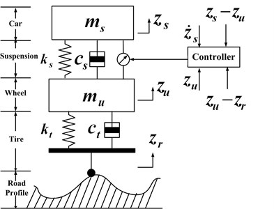
Consider a simplified nonlinear vehicle suspension shown in Fig. 1 [3, 4, 8, 9]. The dynamic equation can be expressed as:
where and denote the sprung mass and unsprung mass, receptively; and are the stiffness and damping of vehicle passive suspension; denotes the compressibility of the pneumatic tire; and are the nonlinear parameters. and stand for the displacements of the sprung mass and unsprung mass, respectively. denotes the external road displacement acting on the active suspension, and represents the active control force generated from the hydraulic pressure or electromagnetic equipment.
As it is well known, the performance criteria of ride comfort, road holding ability, and suspension deflection must be taken into consideration while designing the vibration control strategy for nonlinear vehicle active suspension. The sprung mass acceleration , suspension deflection , and tire deflection must be small enough to improve the ride comfort, prevent from the excessive suspension bottoming, and obtain the good road holding, respectively. Therefore, the controlled output can be defined as:
Introducing the following state variables as:
and defining:
the space state expression of nonlinear active vehicle suspension can be constructed as:
where:
Fig. 1Simplified vehicle active suspension
Road disturbance is considered as vibration caused by road roughness [3-5, 8]. As stated in [3, 8], the road disturbances can be derived from a random process with ground displacement power spectral density (PSD):
where denotes a spatial frequency, is a reference frequency. The value of denotes the measurement for the road roughness, where and are the roughness constants.
The road displacement input from road irregularities in Eq. (1) can be written as:
where , is the length of a road segment, is a random variable, , and can restrict the frequency range of a vehicle body. Then, the road disturbance can be described as:
The following state space vectors are defined as:
Then the road disturbance input can be formulated as the output of a random linear exogenous system with an unknown initial value:
where is the state vector with unknown initial value the expressions of and are represented as:
where and is the constant horizontal velocity. Positive integer limits the considered frequency band lower than 20 Hz in road disturbances Eq. (8).
Defining as the sampling period, the discrete expression of Eq. (5) can be given by:
where , , , and .
Meanwhile, the discrete form of exogenous system Eq. (11) can be described as:
where .
In order to trade off among the various performance requirements, the following quadratic average performance index is chosen as:
where is a positive semi-definite matrix, is a constant.
In what follows, we will discuss how to design the DAOVC for system Eq. (5) subject to road disturbances (14) such that the quadratic average performance index Eq. (15) reaches its minimum value. The following assumptions and lemma are given first.
Assumption 1: The triple is completely controllable-observable.
Assumption 2: The nonlinear vector function in Eq. (5) is piecewise continuous in with satisfying Lipschitz conditions on and , where is a positive integer related to .
Assumption 3: The exogenous system Eq. (14) is stable, i.e., for any , where denotes the eigenvalues of matrix .
Lemma 1: [16] Let and The matrix equation:
has a unique solution if and only if:
where are eigenvalues of matrix.
3. Design of procedure for DAOVC
3.1. Original nonlinear TPBV problem
Applying the maximum principle to the vibration control problem for Eqs. (13) and (14) with respect to the performance index Eq. (15), a nonlinear TPBV problem can be formulated as:
where denotes a Jacobian matrix of with respect to , , , and
Then, the optimal vibration controller can be expressed as:
However, it is difficult to obtain the analytical solution of TPBV problem Eq. (18) caused by nonlinear items and . Therefore, we will design a procedure for solving the nonlinear TPBV problem Eq. (18) to obtain DAOVC.
3.2. Reformation of original nonlinear TPBV problem
By introducing a sensitive parameter , the nonlinear TPBV problem Eq. (18) can be formulated as:
Meanwhile, the optimal vibration control law Eq. (19) can be reconstructed as:
It is assumed that , , , , and are differentiable at , and their Maclaurin series are described as:
where . While 1, the formulated TPBV problem Eq. (20) is equivalent to nonlinear TPBV problem Eq. (18).
Then, the formulated TPBV problem Eq. (20) can be rewritten as:
The following sequence of TPBV problems can be obtained:
From Eq. (20) and Eq. (21), one yields:
It should be pointed that DAOVC can be obtained by integrating with Eq. (24), with Eqs. (25), and (26).
Remark 1: For the step, the nonlinear item and can be calculated from the th step. Therefore, the series Eq. (26) can be calculated from the sequence of Eqs. (24) and (25).
3.3. Design of DAOVC
In this subsection, we will propose the designed DAOVC and prove its existence and uniqueness. We give out the following theorem.
Theorem 1: Consider the vibration control problem for discrete nonlinear vehicle active suspension Eq. (13) subject to road disturbance Eq. (14) with respect to the quadratic average performance index Eq. (15), the DAOVC is existent and unique, which can be expressed as:
where ; is the unique positive-definite solution of the Riccati equation:
is the unique solution of the following Stein equation:
and the nonlinear compensation can be obtained from:
where the sequence of can be calculated from:
Proof: First, we will discuss the solution of . Defining as:
and substituting Eqs. (32) into (26), one gets:
Then the in the 0th sequence can be described as:
From Eqs. (24), (32), and (34), we have:
Substituting Eq. (35) into the second formula in Eq. (24), one gets:
Comparing the coefficients between Eq. (32) and Eq. (36), Riccati Eq. (28) and Stein Eq. (29) can be obtained. Then, the can be computed.
Next, we will discuss the solution of. Introducing the following as:
and substituting the first formula of Eq. (21) into , one gets:
From Eqs. (26) and (37), the in the th sequence can be described as:
Then one yields:
Based on Eq. (40) and the second formula of Eq. (25), we have:
Comparing the coefficients between Eqs. (37) and (41), the nonlinear compensation Eq. (30) can be obtained. From of Eq. (34), of (39), and , the DAOVC can be obtained as Eq. (27).
Finally, the existence and uniqueness of DAOVC Eq. (27) will be proved. Actually, it is equivalent to prove the existence and uniqueness of the matrices and, respectively.
Based on the Assumption 1 that the triple is completely controllable-observable and the optimal control theory, the positive-definite matrix is the existence and uniqueness solution of Eq. (29). The solution of nonlinear compensation Eq. (30) can be described as:
Based on Assumption 1, one has:
From Assumption 2 and Eq. (43), we have:
Then is the existent and unique solution of Stein Eq. (30) based on Lemma 1. Therefore, the proposed DAOVC Eq. (27) is the existence and uniqueness. The proof is completed.
3.4. Computational realizability of DAOVC
We can easily discover that it is impossible to obtain the vibration control law Eq. (27) caused by the infinite item . In order to make the result more practical, a positive integer can be decided to replace the in Eq. (27). Then DAOVC Eq. (27) can be reformed as:
An iteration formula for DAOVC can be obtained:
In order to decide the value of , the following iteration algorithm is proposed based on the control performance in each iteration procedure, which is described as
Step 1: Set a small positive number; let and ; calculate the values of , and from Eqs. (28), (29) and the first formula of Eq. (46), respectively;
Step 2: Substitute into discrete vehicle active suspension Eq. (13); calculate the value of performance index Eq. (15) for the th iteration procedure based on:
Step 3: If , then define , obtain the DAOVC law , and stop;
Step 4: Else set ; obtain based on Eq. (30) and compute by replacing into the second formula of Eq. (46), go to Step 2.
4. Numerical example
The parameters of vehicle active suspension are listed as [4, 8]: the sprung mass is 972.2 kg, the unsprung mass is 113.6 kg, the damping and stiffness of the vehicle passive suspension are 1095 Ns/m and42719.6 N/m; the compressibility of the pneumatic tire is 10115 N/m; the nonlinear parameters and . Defining the sampling period as 0.08 s, the following matrices in Eq. (13) can be obtained:
Under the road disturbances with 20 m/s, 400 m, 2, 1.5, and road roughness 256×10-6 m3, the road displacement input can be generated from Eq. (14). Then, the road curve of road disturbances is depicted in Fig. 2.
Let the weight matrices in Eq. (11) be and 1. In order to illustrate the effectiveness of the proposed DAOVC, the classical FFOVC is used to compare with the proposed DAOVC, which is described as:
Setting the small positive number 0.001, we obtain that the control performance in 5th iteration procedure satisfies . This means that the DAOVC in the 5th iteration satisfies with the requirement of proposed iteration algorithm. Meanwhile, the control performances under the OL system and FFOVC are 3.584×10⁵ and 3.491×10⁴, respectively. The control performance values in each iteration are listed in Table 1, and the reduction percentage is displayed compared with that of OL system.
Table 1Control performance under DAOVC and FFOLVC
Iterative time M | 1 | 2 | 3 | 4 | 5 |
Control performance | 9.232×10⁴ | 7.343×10⁴ | 6.125×10⁴ | 3.951×10⁴ | 3.948×10⁴ |
Reduction percentage | 72.24 % | 79.51 % | 82.91 % | 88.98 % | 88.98 % |
Fig. 2Curve of road disturbances
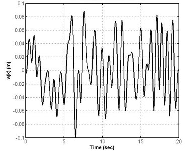
Fig. 3Curves of DAOVC and FFOVC
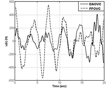
The covers of the FFOVC and proposed DAOVC are shown in Fig. 3. The response curves and frequency spectrums of the sprung mass acceleration (SMA), sprung deflection (SD), and tire deflection (TD) are shown in Figs. 4-6 under the open-loop (OL) system, DAOVC, and FFOVC, where the parts (a) show the response curves, and the parts (b) show the frequency spectrums. Meanwhile, in order to show the effectiveness of the proposed DAOVC clearly, the peak values and root-mean square (RMS) values of SMA, SD, and TD are shown in Table 2 compared with ones under the OL systems and FFOVC.
The peak values of DAOVC and FFOVC are 405.9 and 550, respectively. The RMS values of DAOVC and FFOVC are 146.7 and 237.1, respectively. Therefore, from Fig. 3, it can be seen clearly that the value of DAOVC is smaller than that of FFOVC. At the same time, the curve of DAOVC is smoother than that of FFOVC. It indicates that the consumption of DAOVC is smaller than that of the classical FFOVC.
Fig. 4Curves and frequency spectrum of SMA under OL system, DAOVC law, and FFOVC
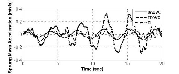
a) SMA under different control law
b) Frequency spectrums of SMA under different control law
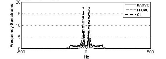
Fig. 5Curves and frequency spectrum of SD under OL system, DAOVC law, and FFOVC
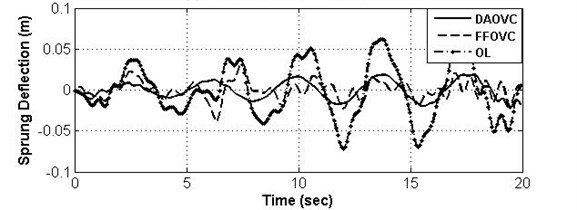
a) SD under different control law
b) Frequency spectrums of SD under different control law
In what follows, we will discuss the control performance under DAOVC and FFOVC.
From the curves of SMC, SD, and TD shown in the (a) parts of Figs. 4-6, it can be seen that the values of SMA, SD, and TD under DAOVC can be converted to smaller values than those under the OL system and FFOVC. Meanwhile, the curves of SMA, SD, and TD under proposed DAOVC are smoother than those of OL system and FFOVC. Specially, under the DAOVC law, the peak value of SMA is reduced to about 70.23 % compared to that of OL system, the RMS value of the sprung mass acceleration is reduced to about 66.76 %, the RMS of sprung deflection is reduced to about 67.37 %, and the RMS of tire deflection is reduced to about 72.30 % less than that of OL system. It indicates that the proposed DAOVC can improve the performance requirements of ride comfort, road holding ability, and suspension deflection more effectively. Therefore, it can be concluded that the control performance can be improved, and the nonlinear response can be compensated effectively under the proposed DAOVC.
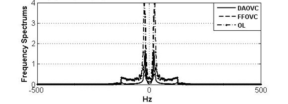
Fig. 6Curves and frequency spectrum of TD under OL system, DAOVC law, and FFOVC
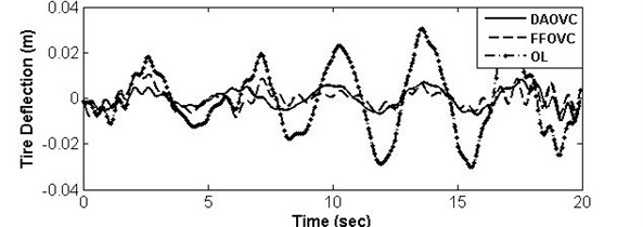
a) TD under different control law
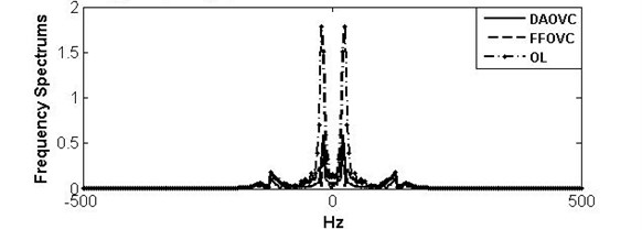
b) Frequency spectrums of TD under different control law
Table 2Peak and RMS values of performance criteria and controller under DAOVC and FFOLVC
Name | SMA | SD | TD | (102) | |
Peak values | OL | 3.215 | 0.649 | 0.306 | \ |
DAOVC | 0.957 (–70.23) | 0.185 (–71.49) | 0.081 (–73.53) | 4.059 | |
FFOLVC | 1.161 (–63.88) | 0.329 (–49.31) | 0.107 (–65.03) | 5.500 | |
RMS values | OL | 1.483 | 0.331 | 0.148 | \ |
DAOVC | 0.493 (–66.76) | 0.108 (–67.37) | 0.041 (–72.30) | 1.467 | |
FFOLVC | 0.558 (–62.37) | 0.151 (–49.95) | 0.074 (–50.00) | 2.371 | |
Meanwhile, from the frequency spectrums of SMA, SD, and TD shown in the (b) parts of Figs. 4-6, the frequencies of SMA, SD, and TD are dispersed in the range [–20, 20] Hz under DAOVC. On the contrary, the frequency ranges under OL systems and FFOVC are wider than that of DAOVC. It indicates that the vibration frequencies of SMA, SD, and TD are restrained by DAOVC. It indicates that the vibration of vehicle body is eliminated effectively. Therefore, the vibration of suspension vehicle caused by road disturbance can be eliminated significantly by using the proposed DAOVC.
From Tables 1-2 and Figs. 3-6, it can be found that the designed DAOVC can effectively compensate the nonlinear responses and offset the vehicle body’s vibration caused by road disturbances. Meanwhile, the control performance of nonlinear vehicle active suspension can be improved significantly under DAOVC.
5. Conclusions
In this paper, the optimal vibration control problem for nonlinear vehicle active suspension was discussed. The vibration control problem was reformed as a nonlinear TPBV problem first. By introducing a sensitive parameter and using the Maclaurin series, the DAOVC was devised by solving a Riccati equation, Stein equation, and a nonlinear compensation. Also, an iteration algorithm was designed to realize the computational realizability of DAOVC. From simulation results, the values of SMA, SD, and TD can be converted to smaller ones by using the proposed DAOVC, and control performance can be improved effectively.
References
-
Tseng H. E., Hrovat D. State of the art survey: active and semi-active suspension control. Vehicle System Dynamics, Vol. 53, Issue 7, 2015, p. 1034-1062.
-
Sun X. Q., Chen L., Wang S. H. Damping multi-model adaptive switching controller design for electronic air suspension system. Journal of Vibroengineering, Vol. 17, Issue 6, 2015, p. 3211-3223.
-
Han S.-Y., Tang G.-Y., Chen Y.-H., Yang X.-X., Yang X. Optimal vibration control for vehicle active suspension discrete-time systems with actuator time delay. Asian Journal of Control, Vol. 15, Issue 6, 2013, p. 1579-1588.
-
Du H., Zhang N. H∞ control of active suspension with actuator time delay. Journal of Sound and Vibration, Vol. 301, 2007, p. 236-252.
-
Brezas P., Smith M. C. Linear quadratic optimal and risk-sensitive control for vehicle active suspensions. IEEE Transactions on Control Systems Technology, Vol. 22, Issue 2, 2014, p. 543-566.
-
Zhang M., Nie H., Zhu R. Stochastic optimal vibration control for flexible aircraft taxing at constant or variable velocity. Nonlinear Dynamics, Vol. 62, Issues 1-2, 2010, p. 485-497.
-
Gohrle C., Schindler A., Sawodny O. Design and vehicle implementation of preview active suspension controller. IEEE Transactions on Control System Technology, Vol. 22, Issue 3, 2014, p. 1135-1142.
-
Lei J., Jiang Z., Li Y., Li W. Active vibration control for nonlinear vehicle suspension with actuator delay via I/O feedback linearization. International Journal of Control, Vol. 87, Issue 10, 2014, p. 2081-2096.
-
Sun W., Pan H., Zhang Y., Gao H. Multi-objective control for uncertain nonlinear active suspension systems. Mechatronics, Vol. 24, Issue 4, 2014, p. 318-327.
-
Bououden S., Chadli M., Karimi H. R. Robust predictive control design for nonlinear active suspension systems. Asian Journal of Control, Vol. 18, Issue 1, 2016, p. 122-132.
-
Li H., Yu J., Hilton C., Liu H. Adaptive sliding-mode control for nonlinear active suspension vehicle systems using T-S fuzzy approach. IEEE Transaction on Industrial Electronics, Vol. 60, Issue 8, 2013, p. 3328-3338.
-
Liu S., Zhou H., Luo X., Xiao J. Adaptive sliding fault tolerant control for nonlinear uncertain active suspension systems. Journal of the Franklin Institute, Vol. 353, Issue 1, 2016, p. 180-199.
-
Cetin S. Adaptive vibration control of nonlinear quarter car model with electromagnetic active suspension. Journal of Vibroengineering, Vol. 17, Issue 6, 2015, p. 3063-3078.
-
Han S.-Y., Wang D., Chen Y.-H., Tang G.-Y., Yang X.-X. Optimal tracking control for discrete-time systems with multiple input delays under sinusoidal disturbances. International Journal of Control, Automation, and Systems, Vol. 13, Issue 2, 2015, p. 292-301.
-
Peng C., Han Q., Yue D. A delay system method for designing event-triggered controllers of networked control systems. IEEE Transactions on Automatic Control, Vol. 58, Issue 2, 2013, p. 475-481.
-
Sujit K. M. The matrix equation AXB+CXD=E. SIAM Journal on Applied Mathematics, Vol. 32, 1977, p. 823-825.
About this article

This work was supported by the National Natural Science Foundation of China under Grant (51277116, 61573166), the Program for Scientific Research Innovation Team in Colleges and Universities of Shandong Province, Shandong Provincial Natural Science Foundation under Grant ZR2015JL025, and Shandong Distinguished Middle-Aged and Young Scientist Encourage and Reward Foundation Grant BS2014DX015.
