Application of CBSR and LMD in reciprocating compressor fault diagnosis

1. Introduction

Concern about mechanical condition monitoring and fault diagnosis has been attracting widespread interest in recent years. Much research has been focused on signal processing technique and fault feature extracting method. However, since the reciprocating compressor often works in harsh environment, it will lead to the measured vibration signal with a low signal to noise ratio, representing weak features and serious noise pollution [1].

Therefore, in the early fault stage of the equipment, the modulation characteristic of signals tend to be overwhelmed, as a result, it is difficult to fulfill the early fault detection. A major current focus in weak feature extraction methods is attempting to eliminate or suppress the noise of the signal. Unfortunately, the fault modulation characteristics of vibration signal are also weaken with the denoising process. In order to overcome the weakness of the traditional denoising methods, stochastic resonance (SR) was proposed by Benzi R. [2], which utilized the input signal noise in nonlinear system to obtain a resonance output. With the synergistic effect of nonlinear system, SR method can transfer energy from high frequency to low frequency, strengthening the modulation characteristic while weakening the signal noise. SR method has been widely used to extract weak signal in strong background noise. For instance, Zhao Y. responded to the need for increased denoising performance by introducing cascaded bistable stochastic resonance (CBSR) [3], the phenomenon that the energy of noise in high frequency was gradually decreased while the energy of the low-frequency modulation signal was progressively strengthened was described in detail. Hence CBSR is suitable to extract the weak fault feature from the strong noisy environment. Due to the direct relationship between the vibration and structure of the machinery, the vibration signal has been widely applied in the reciprocating compressor fault diagnostic field.

Since the reciprocating compressor fault vibration is a multi-component, amplitude-modulated (AM) and frequency-modulated (FM) signal, much research has focused on the time-frequency processing methods, such as window fourier transform, wavelet transform [4] and the Hilbert-Huang transform (HHT) [5] and so on. However, the traditional signal processing methods have their own limits. Take windowed Fourier transforms (WFT) for example, once the window function is fixed, the size of the time-frequency window is unchangeable. Wavelet transform (WT) can decompose a multi scales into several scale time-frequency components, which has the ability of processing the non-stationary and non-linear signals. WT has been widely used to diagnostic the machinery. However, WT is essentially an adjustable window Fourier transform in fact, which doesn’t have the nature of self-adaptive feature [6].

Empirical mode decomposition method (EMD) [7] can self-adaptively decompose a complicated signal into a series of intrinsic mode functions (IMFs), which is completely a self-adaptive signal processing method. Combined with Hilbert transform, we can obtain the instantaneous amplitude (IA) and instantaneous frequency (IF). Although EMD has become an established tool for the non-stationary and non-linear signals analysis, the mode mixing, end effect and over- and undershoot envelope fitting problems also limit its applications. Furthermore, the Hilbert transform can often result in doubtful negative IA. In this paper, we put forward a novel adaptive time-frequency analysis method called local mean decomposition (LMD), which is proposed by Jonathan S. Smith and successfully used in EEG field [8]. LMD can decompose a superimposed signal into a complex series of product functions (PFs) and a residual. Each PF component is the product of an envelope signal $a\left(t\right)\mathrm{}$and a pure frequency modulation (FM) signal $s_n\left(t\right)$. Therefore, LMD method can adaptively decompose any multi-component signal into several single-component AM-FM signals [9]. It is generally accepted that the reciprocating compressor vibration signals measured by sensor often represent multi-component, AM-FM features, simultaneously a sum of mono-component can be obtained by applying LMD method. Hence, LMD is suitable to process the reciprocating compressor vibration signals. In the original LMD algorithm, moving average (MA) approach is performed to construct the local mean function and envelope functions in the sifting process, which may pose a major problem for LMD. Since unsuitable sliding step sizes of MA has an adverse impact on the final calculation of IA and IF in the end [10]. Therefore, the selection of the sliding step is also a challenge problem. Furthermore, the MA approach is time-consuming in the actual time series analysis, and there remain need for an efficient method that can perform the decomposition accurately and efficiently. To overcome the drawbacks of original LMD, in this paper the Hermite interpolation is adopted to construct the local mean function and envelope functions [11].

Naturally, by virtue of the advantages of CBSR and Hermite-LMD, a reciprocating compressor fault diagnosis method based on CBSR denoising and Hermite-LMD is put forward. CBSR system has the merits of transforming the energy from noisy signal with high-frequency to modulation signal with low frequency, eliminating the impact of noise on LMD decompose effectively. Hermite-LMD can obtain more accurate decomposition results by performing Hermite interpolation to calculate the extremum envelope. Finally, the simulation and experiment results demonstrate that the proposed method is effective for analysis of highly non-stationary and non-linear vibration signal.

The rest of this paper is organized as follows: Section 2 describes the CBSR method and the main steps of hermite-LMD. In addition, the procedures of proposed CBSR and hermite-LMD are introduced briefly. The simulation signals analysis of the proposed method is given in Section 3. The applications of reciprocating compressor fault diagnosis are shown in Section 4. Finally, the conclusions about the diagnostic capability of the proposed method are drawn in Section 5.

2. The proposed method based on CBSR and Hermite-LMD

2.1. Hermite-LMD algorithm and problems

LMD method can decompose a multi-component signal into a series of PF components and a residual. Each PF component is the product of an envelope signal $a\left(t\right)$ and a pure FM signal $s_n\left(t\right)$. Envelope signal is the product of the IA and IF, which is calculated by the pure FM signal $s_{in}\left(t\right)$ according to Eq. (4):

1

$f_i\left(t\right)=\frac{1}{2\pi }\frac{d\left(\mathrm{a}\mathrm{r}\mathrm{c}\mathrm{c}\mathrm{o}{\mathrm{s}}_{in}\left(t\right)\right)}{dt}.$

In the traditional LMD method, the local mean function $m\left(t\right)$and envelope estimation function $a\left(t\right)$ are constructed by using MA approach in the sifting process. Whereas the inappropriate sliding step sizes of MA has an adverse impact on the final calculation of IA and IF in the end. Therefore, the selection of the sliding step is a major problem [10]. Since the cubic spline interpolation has good convergency and high smoothness, Hu J. introduced the cubic spline interpolation method to construct the local mean function $m\left(t\right)$and envelope estimation function $a\left(t\right)$ [14]. However, the cubic spline interpolation is performed to construct the envelopes with outstanding over- and undershoot problems [15]. Recently cubic Hermite interpolation method is found optimum in the post treatments of CBSR [11]. The cubic Hermite interpolation method is widely used in engineering, which has a continuous first derivative property at the node. Therefore, the points are continue and smooth, and the line has an excellent conformal characteristic. Since the reciprocating compressor vibration signal is non-stationary and nonlinear, the cubic Hermite interpolation is suitable for fitting envelope of the vibration signal. Firstly, find out all the extreme points of the signal, and then fit upper envelope $E_{up}\left(t\right)$ and lower envelope $E_{low}\left(t\right)$ by using cubic Hermite interpolation, respectively. Then local mean function $m\left(t\right)$ and envelope estimation function $a\left(t\right)$ can be obtained by Eq. (5) and Eq. (6):

2

$m\left(t\right)=\frac{E_{up}\left(t\right)+E_{low}\left(t\right)}{2},$

3

$a\left(t\right)=\frac{\left|E_{up}\left(t\right)-E_{low}\left(t\right)\right|}{2}.$

After obtaining the local mean function $m\left(t\right)$ and envelope estimation function $a\left(t\right)$, we continue to perform the following steps of LMD to fulfill the Hermite-LMD signal processing approach.

However, the noise in vibration signals will increase the number of PFs and the strong noise even give rise to aliasing of a fault signal and the noise signal. To make further explanation, we take a simulation signal to demonstrate the noise effect to LMD decomposition. Here, a simulation signal $x\left(t\right)$ is given as follows: $x\left(t\right)=0.5\left(\mathrm{s}\mathrm{i}\mathrm{n}\left(10\pi t\right)\right)+\mathrm{s}\mathrm{i}\mathrm{n}\left(30\pi t\right){\mathrm{e}}^{t/2}$. Set the sampling frequency 1000 Hz and $t=$ 0:1/1000:3.

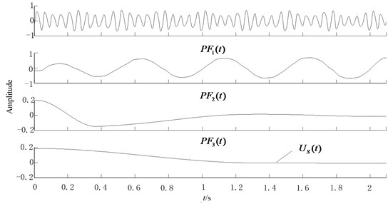
The waveform of the signal $x\left(t\right)$ and the LMD decomposition results are shown in Fig. 1(a). As can be seen, the original signal is decomposed into two PF components and a residual, $P{F}_1\left(t\right)$ and $P{F}_2\left(t\right)$ are corresponding to the simple components $x_1\left(t\right)=\mathrm{s}\mathrm{i}\mathrm{n}\left(30\pi t\right){\mathrm{e}}^{t/2}$ and $x_2\left(t\right)=0.5\left(\mathrm{s}\mathrm{i}\mathrm{n}\left(10\pi t\right)\right)$ in the original signal $x\left(t\right)$, respectively. There is no mode mixing phenomenon happened in the obtained PF components, which match the true components well.

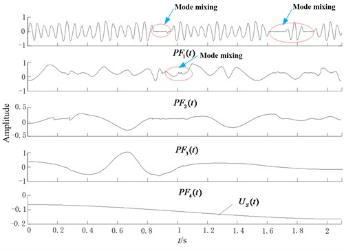
To demonstrate the effect of noise to the decomposition performance, the white noise is added to the signal $x\left(t\right)$, then LMD is also applied to decompose the noisy signal, the waveform of the noisy signal and decomposition results are shown in Fig. 1(b). As we can see, four PF components are obtained and there are notable abnormal distortion happened in the PF components, resulting in imprecise decomposition results.

In the real measured vibration signals of mechanical system, the background noise is unavoidable. Hence, it is necessary to weaken the noise in the signal before we conduct the LMD decomposition. In this paper, CBSR method is introduced to preprocess the noisy signals, which can weaken the noise progressively while strengthen the weak fault periodic signal [12]. The noisy signal processed by CBSR can not only eliminate the impact of noise on the LMD but also improve the decomposition quality of LMD. The detailed procedures of CBSR will be described in Section 2.2.

Fig. 1LMD decomposition results of the signal x(t)

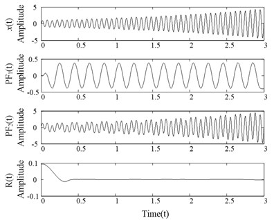
a) LMD results of the signal $x\left(t\right)$ without noise

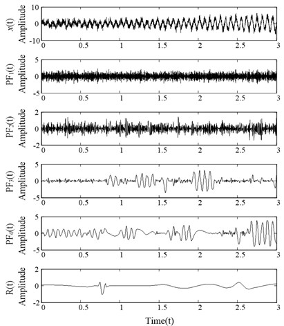
b) LMD results of the noisy signal

2.2. Cascaded bistable stochastic resonance

2.2.1. The theorem of bistable stochastic resonance

Bistable stochastic resonance systems are outlined later [13]. Firstly, when the system is driven by a small periodic signal, the outputs of system can’t occur energy transitions. With the noise intensity increasing, the energy transition is happening under the common action of the weak noisy signal and a small periodic signal.

Stochastic resonance system is composed of nonlinear system, periodic signal $s\left(t\right)$ and noise signal $n\left(t\right)$. It is generally described by using Langevin equation as follows:

4

$\frac{d_x}{d_t}=ax-b{x}^3+S\left(t\right)+n\left(t\right),$

where $a$, $\mathrm{b}$are non-zero real numbers; $S\left(t\right)$ is a periodic signal, expressed as $S\left(t\right)=A\mathrm{c}\mathrm{o}\mathrm{s}\left(2\pi ft\right)$; $A$ is amplitude; $f$ is frequency; $n\left(t\right)$ is a Gaussian white noise, satisfied with the average statistical properties $E\left[n\left(t\right)\right]=0$:

5

$E\left[n\left(t\right)n\left(t^{\text{'}}\right)\right]=2D\delta \left(t-t^{\text{'}}\right),$

where $D$ is noise intensity, $\delta \left(t\right)$ is impulse function.

If $A=D=0$, in fact, there is not the driving force or external periodic noise, we can obtain:

6

$V\left(t\right)=-\frac{a}{2}{x}^2+\frac{b}{4}{x}^4.$

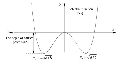
As can be seen in Fig. 2, bistable potential function has a maximum and two minima when $x=0$ and $x=\pm \sqrt{a/b}$, corresponding to a barrier point and two traps, the barrier depth $\mathrm{\Delta }V=V\left(0\right)-V\left(x_{\pm }\right)=a^2/4b$. When given a periodic weak signal system $S\left(t\right)$, signal can’t break through the barrier of $\mathrm{\Delta }V$. When given a noisy signal $n\left(t\right)$, part of the noise energy translates to the periodic signal. With period signal and noisy signal driving at the same time, they can overcome the barrier of $\mathrm{\Delta }V$ and the energy transition occurs between the two steady state signals, resulting in the phenomena of resonance.

Fig. 2Bistable system potential pitfalls diagram

The sampling frequency is so high that can’t satisfy small parameter requirements of the adiabatic elimination theory of stochastic resonance (SR) [12]. In this paper, we adopt twice sampling stochastic resonance to detect a weak signal overwhelmed in strong background noise. The twice sampling stochastic resonance can be briefly summarized as follows. Firstly, resample the large parameter signal and compress linearly from high to low, therefore, it becomes a small parameter signals. Then the obtained signal is taken as inputs of SR system and carried out a treatment of resonance. Finally, amplify the processed data in compressed scale to achieve a large parameter signal. Through the procedures mentioned above, SR could apply in large parameters practical analysis with the help of twice sampling.

2.2.2. CBSR system

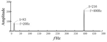
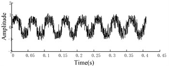
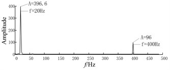
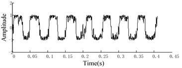
CBSR system is cascaded by individual bistable SR in the order of around, the procedure is shown in Fig. 3. The output signals in bistable SR system has the characteristic of Lorentz distribution, in which not only high frequency noise is efficiently removed but also low frequency signals is enhanced. Noisy signals and CBSR output are shown in Fig. 4. Fig. 4(a) gives the noisy signal, which is composed of two sinusoidal signals. The frequencies of two sinusoidal signals are 20 Hz and 400 Hz, respectively, which is shown in Fig. 4(b).

Figs. 4(c), (e) and (g) illustrate time-domain waveforms given by CBSR system in the first, second and third grade. Also the corresponding spectrums are shown in Fig. 4(d), (f) and (h), respectively. In comparison with Fig. 4(b) with (d), (f) and (h), it can be found that the energy transfer mechanism from high frequency area to low frequency area. Compared Fig. 4(a) with Figs. 4 (c), (e) and (g), the conclusions can be got that the output waveform exhibits smooth gradually as the high frequency components are consecutively removed. The simulation demonstrates that an effective low pass filter can be achieved by using CBSR system.

Fig. 3CBSR system

2.3. The procedure of the proposed method

In order to improve the quality of LMD decomposition, firstly, the noisy signal is taken into CBSR system and then the denoised signal is decomposed by LMD. The detailed steps are as follows:

1) Resample the original signal $x\left(t\right)$ with noise so as to satisfy the requirements of the stochastic resonance adiabatic small parameter.

2) The small parameter signal is fed into CBSR system to remove the noisy, generating $x_n\left(t\right)$.

3) Restore $x_n\left(t\right)$ to the sampling frequency of the original signal.

4) Get the extreme point sequence $n_k$ from$\mathrm{}{x}_n\left(t\right)$, extend endpoints to obtain a new extreme point sequence $X_k$.

5) From one side of $X_k$, choose the adjacent extreme points and fit upper envelope $E_{up}\left(t\right)$ and lower envelope $E_{low}\left(t\right)$ with cubic Hermite interpolation.

6) Calculate local mean function $m\left(t\right)$ and envelope estimation function $a\left(t\right)$ according to Eq. (5) and Eq. (6).

Fig. 4Noisy signals and CBSR output

a)The waveform of original signal

b) The spectrum of noisy signal

c) The waveform of SR outputs of grade 1

d) The spectrum of SR outputs of grade 1

e) The waveform of SR outputs of grade 2

f) The spectrum of SR outputs of grade 2

g) The waveform of SR outputs of grade 3

h) The spectrum of SR outputs of grade 3

Then continue the following steps of LMD to realize the CBSR and hermite-LMD method. A flowchart of the proposed method is shown in Fig. 5.

In addition, in the practical applications, the parameter $\delta$ can be introduced to stop the iteration process. Namely, when $a_{ij}\left(t\right)$ in the flowchart satisfies ${1-\delta \le a}_{ij}\left(t\right)\le 1+\delta$, the iteration can be stopped.

3. Simulation analysis

In this section, a simulation signal $x\left(t\right)$ is constructed to valid the effectiveness of the CBSR denoising, which consists of an AM signal $x_1\left(t\right)$, an FM signal $x_2\left(t\right)$ and a white noise, set sampling frequency 1000 Hz, the sampling points is 2048. The waveforms of noisy signal are shown in Fig. 6(a):

Fig. 5A flowchart of the CBSR denoising and Hermite interpolation LMD

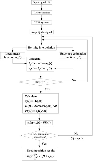
Fig. 6Waveforms of noisy signal and CBSR outputs

a) Waveforms of noisy signal

b) Waveforms of the first CBSR output

c) Waveforms of the second CBSR output

The parameters of CBSR method are set as follows: the twice sampling frequency is 5 Hz and the parameters of stochastic resonance parameters are $a=$ 0.1, $b=$ 1. Also, in this paper, the second order SR is adopted to remove the noise.

To begin with, CBSR method is used to process the noisy signal in Eq. (7). The results of the first and second CBSR output are shown in Fig. 6 (b) and Fig. 6(c), respectively. As can be seen, there is some burr in the original signal, after the process of CBSR, the high frequency is eliminated gradually, simultaneously, the signal becomes smoother. Then, Hermite-LMD is performed to decompose the denoised signal.

To show the superiority of CBSR and Hermite-LMD method, the noisy signal and the wavelet denoised signal are also combined with Hermite-LMD method to analyze the same simulation signal. In addition, the boundary conditions of the simulation signal have been handled by the mirror-symmetric extension. The iteration stop condition of LMD is ${1-\delta \le a}_{ij}\left(t\right)\le 1+\delta$, where $\delta ={10}^{-4}$.

The LMD decomposition results are shown in Fig. 7, Fig. 8 and Fig. 9.

Fig. 7LMD results of noisy signal

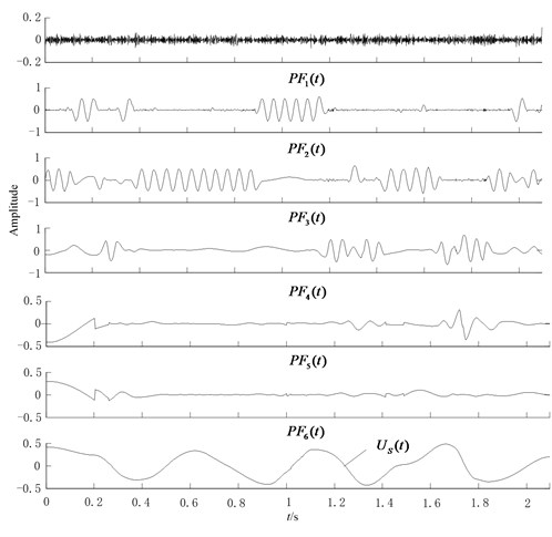
Fig. 8Hermite-LMD results of the wavelet output

As can be seen in Fig. 7, the Hermite-LMD decomposition results of noisy signal are serious distorted. Fig. 8 shows the Hermite-LMD decomposition results of wavelet denoised signal. It consists of 5 PFs and a residual. PF1 is the FM signal $x_2\left(t\right)$ and PF2 is the AM signal $x_1\left(t\right)$. Although, wavelet denosing approach improves the decomposition performance, there is still some mode mixing and distortion occurs in the PF1 and PF2 components. Fig. 9 gives the hermite-LMD decomposition results of CBSR denoised signal. As can be seen, 3 PF components and a residual are obtained, the high frequency is mostly removed, and it can be obviously found out the FM signal corresponding to PF1 and the AM signal corresponding to PF2 without the mode mixing phenomenon.

The simulation demonstrates CBSR can reduce the decomposition layers and improve the decomposition accuracy of LMD effectively, in comparison with the directly using LMD and wavelet denoising method.

Fig. 9Hermite-LMD results of the CBSR output

4. Engineering applications

It is generally accepted that the envelope analysis technique is appropriate to extract the fault feature from the measured vibration signals [16]. When the reciprocating compressor with local fault operates, the measured vibration signal is a multi-component, amplitude-modulated (AM) and frequency-modulated (FM) signal, and the amplitude of the high frequency is modulated by the shock impulse, which is generated by the local fault. Since the reciprocating compressor fault vibration has the characteristics of multi-component, AM and FM, the LMD method can decompose a complicated signal into a series of PFs adaptively. Therefore, LMD method is especially suitable for processing the reciprocating compressor fault signal and a new fault diagnosis technique based on CBSR and Hermite-LMD is proposed. The proposed method can be summarized as follows. Firstly, the CBSR is taken as a pretreatment to eliminate noise with the help of the good denoising performance. Then the output signal of CBSR can be decomposed into a set of mono-component PFs by using LMD method. Finally, the spectrum analysis is applied to first PF component to extract the modulated feature.

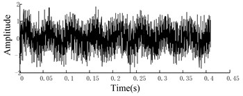
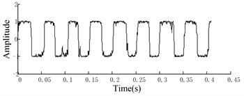
In order to validate the effectiveness of the proposed method, the proposed method is applied to fulfill fault diagnosis of reciprocating compressor. The experiment was conducted on the double – acting reciprocating compressor of 2D12 in a large-scale in Da Qing, China, whose structure is shown in Fig. 10. The location of the accelerometer is on the bottom of slide on the first crosshead, where the fault frequency is easy to find. The working parameter of the reciprocating compressor is listed in Table 1, and the sample frequency is 50000 Hz. To do further research of the fault patterns and identify the work condition of reciprocating compressor, LMD method was applied to analyze the vibration signal.

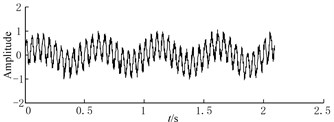
In this experiment, since the shock occurs twice within once reciprocating motion, the fault frequency is the two times of the rotating speed, we can calculate the fault frequency $f=$ 16.53 Hz. The time domain of typical reciprocating compressor fault vibration signal is illustrated in Fig. 11. In addition, set the twice sampling frequency 5 Hz, and the parameter of CBSR is $a=$ 1, $b=$ 1.

Fig. 10The structure of the reciprocating compressor and the sketch of the air valve

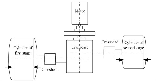
Fig. 11The waveforms of the reciprocating compressor vibration acceleration signal

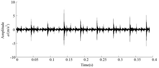
Fig. 12Hermite-LMD decomposition results of original vibration signal

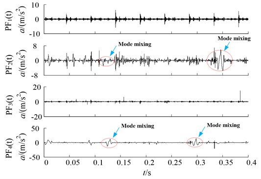
To verify the advantage of the proposed method, a comparison between directly Hermite-LMD decomposition, CBSR and Hermite-LMD is done. Since the PFs with different oscillatory modes are listed from high frequency to low frequency, and the fault information is mainly embedded in the high frequency. For saving space, only the first four PFs are shown in Fig. 12 and Fig. 13, respectively.

By observing the decomposition results of the two methods, the phenomenon of distortion can be easily found in Fig. 12, while there is no such phenomenon occurring in Fig. 13. The comparisons verify the necessity of the signal pretreatment.

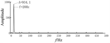
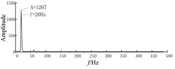
Secondly, the envelope spectrum analysis technique is applied to find the fault frequency ($f=$ 16.53 Hz). Since the fault information is mainly embedded in the high frequency, only the first PF component is selected to perform the envelope spectrum analysis. Fig. 14 and Fig. 15 give the amplitude spectrums of PF1 component obtained by the two methods, respectively. Besides, for clearly comparison, the frequency-axis of all the figures in Figs is amplified by 10 times.

Fig. 13Hermite-LMD decomposition results of the CBSR output

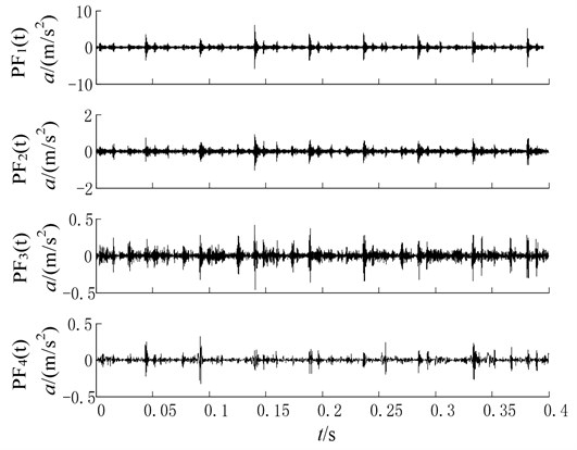
Fig. 14The amplitude spectrums of the PF1 components with CBSR denoising

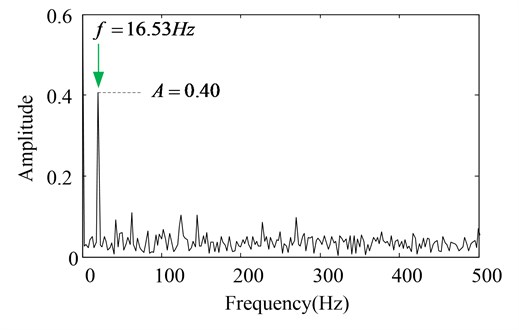
As can be seen in figures, we can find that the fault frequency can be found both in Fig. 14 and Fig. 15. In fact, the appearance of spectra line of $f=\mathrm{}$16.53 Hz is the typical sign of oversized bearing clearance fault, which suggests the reciprocating compressor fault diagnosis has been done. For comparison purpose, although the two methods can identify the fault frequency of roller bearing with ball fault, the envelope spectrum difference of the PF1 components derived from two methods should be discussed. As seen in Fig. 14, the amplitude spectrum has a bigger value with less interference frequency over Fig. 15.

Fig. 15The amplitude spectrums of the PF1 components without CBSR denoising

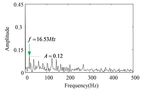
Such phenomenon can be explained by the fact that: the influence of the noise in the reciprocating compressor vibration signal is eliminated by CBSR denoising process, the modulated feature of reciprocating compressor is enhanced simultaneously. Naturally, the denoised signal can improve the decomposition quality of LMD. The comparison results demonstrate that CBSR and Hermite-LMD method can extract more accurate and additional fault signature with less interference frequency over directly using Hermite-LMD method. Hence, the practical reciprocating compressor vibration analysis validate that the combination of CBSR and Hermite-LMD is feasible, which can be used to fulfill fault diagnosis under complex operating condition effectively.

5. Conclusions

In this paper, a new feature extraction method based on CBSR and ermite-LMD is introduced. Firstly, CBSR method is taken as the signal pretreatment method, and then LMD method is performed to decompose the denoised signal. Compared with wavelet denoising, CBSR can not only remove the noisy but also enhance the weak feature, which can improve the accuracy decomposition results of LMD significantly. The effectiveness of the proposed method is validated by the simulation and application to the reciprocating compressor fault diagnosis in comparison with directly LMD method. However, there are many theoretical problems in CBSR, such as the range determination of the twice sampling. Further study will be conducted to investigate the range determination problem.