Analysis, realization and experiment of Lamb wave phased arrays for damage detection and imaging in carbon composite structures

1. Introduction

In order to improve safety and reliability, and to reduce maintenance costs of aerospace structures, development of efficient damage detection and localization techniques is essential [1-4]. Lamb wave can propagate a long distance in plate-like and shell-like structures [5-8]. Hence, structural health monitoring (SHM) [9-13] based on Lamb wave has emerged as a promising technique by using piezoelectric (PZT) actuators/sensors to generate/receive the signals for monitoring the structural damage. The SHM technology is different from the nondestructive examination (NDE) [14] that uses the damage detection strategies to monitor the structural state in real time.

Phased array is an effective damage detection and assessment method in the Lamb wave based SHM system. Comparing to the single sensor identification [15-16], the Lamb wave phased array takes advantage of beam steering to improve the sensitivity. The beam steering of Lamb wave is well controlled to the desired directions by phased array theory. When the wave beam encounters damage in the structure, it generates reflected signal. Previous scholars did a lot of research on phased array based inspection of thin wall structures [17-25]. These researches are not applied on a practical application of engineering.

In this paper, the Lamb wave phased array theory is applied in the structural health monitoring of UAV wing box to identify the damage in the structure. The identification result is shown on the mapped image. The gray level transformation method is used to improve the quality and the contrast of the original damage image. The Lamb wave phased array theory based damage identification and imaging method is verified by using one dimensional PZT linear sensors array to scan and detect the damage and the screw loosening in the carbon composite structures. Meanwhile, the Shannon wavelet is used to calculate the time of arrival of the signals.

2. Phased array based monitoring and imaging theory

Ultrasonic phased array transducer consists of several piezoelectric sensors arranged in a linear array that are independently activated in a sequential manner to scan a certain range of the structure. The signal excited by these PZT sensors array interferes each other in space to form the wave beam-steering focusing on a certain direction. The superposition of ultrasonic wave takes shape in a new wave-front by controlling the phase delay of each excitation signal emitting by PZT array, which is equivalent to changing the location of the transducer. The beam-steering radiated by the PZT array is accordingly changed. And the same rule is implemented in reception of reflection wave. All the signals in the same direction received by PZT array are synthesized and the synthetic signals are shown on the mapped image. Therefore, the ultrasonic phased array can effectively control the direction of wave beam-steering by controlling the phase delay of excitation and reception signal to scan the structure.

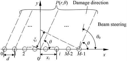
Far-field phased array principle is shown in Fig. 1. The PZT linear array consists of $M$ PZT elements with each PZT element acting as an omni-directional transmitter and receiver. The PZT elements in the array are equally spaced at the distance $d$. The diameter of the PZT element is $d_1$. The coordinate system origin is set to the middle point of the PZT array and the 0° direction is consistent with the alignment of the array. The coordinate in Cartesian coordinate system of $i$th PZT element is ($x_i$, 0), $i=$ 0,…,$M-$1, where $x_i=[i-(M-1)/2]d$.

The phased array principle is applied to generate and receive Lamb waves. For a far-distance point $P(r,\theta )$, the distance $r$ from point $P$ to coordinate system origin is assumed much longer than the PZT element spacing $d$. Because $d\ll r$, the rays connecting the point $P$ with the sensors can be considered with a parallel fascicle of $\theta$. Coordinate system origin is acted as a reference point. For the $i$th PZT element, the distance from the point $P$ to the sensor will be shorted by ${\xi }_i\left(\theta \right)=x_i\mathrm{c}\mathrm{o}\mathrm{s}\theta$. If all the PZT elements are excited simultaneously, the signal from the $i$th PZT element will arrive at point $P$ quicker by ${\delta }_i\left(\theta \right)=x_i\mathrm{c}\mathrm{o}\mathrm{s}\left(\theta \right)/c$. Where $c$ is the Lamb wave group speed traveling in the structure. The total signal received at point $P$ will be:

where $K_1$ is the amplitude attenuation coefficient which the signal travelling from PZT to point $P$, $S_e$ represents excitation signal, and $r/c$ is the time due to the travel distance between the coordinate system origin and the point $P$. Here wave-amplitude conservation is assumed.

If the PZT elements are not excited simultaneously, but with specific time delays $\mathrm{\Delta }{t}_i\left(\theta \right)$ for each PZT element, the total signal received at point $P$ will be:

If $\mathrm{\Delta }{t}_i\left(\theta \right)={\delta }_i\left(\theta \right)$, Eq. (2) becomes:

In this case, the specific time delay for each PZT element is:

Fig. 1Principle of phased array based structural health monitoring

The signal amplitude increases $M$ times in comparison with a single PZT element. The signal-to-noise ratio (SNR) is enhanced. If $\mathrm{\Delta }{t}_i\left(\theta \right)={\delta }_i\left(\theta \right)=x_i\mathrm{c}\mathrm{o}\mathrm{s}\left(\theta \right)/c$, the signal wave-front takes place at angles $\theta$ that is achieved by specific time delays of the exciting signals of the sensors in the linear array.

According to the principle of reciprocity, the receiving process is consistent with exciting process under the same conditions. The point $P(r,\theta )$ acts as a new wave source reflecting the signal to all the PZT elements. The signal arrives the $i\text{th}$ PZT element quicker by ${\delta }_i\left(\theta \right)=x_i\mathrm{c}\mathrm{o}\mathrm{s}\left(\theta \right)/c$. Its expression is:

where $K_1$ is the amplitude attenuation coefficient which the signal travelling from point $P$ to PZT.

The total signal received at all PZT elements from the point $P$ will be:

Hence, with specific time delays $\mathrm{\Delta }{t}_i\left(\theta \right)={\delta }_i\left(\theta \right)$ for each PZT element, the signal reaches to all of the PZT elements at the same time. Its expression is:

where, $K=K_1{K}_2$, $K$ is the total amplitude attenuation coefficient.

Assume that damage exists at angle ${\theta }_0$ and distance $R$ in the structure. The signals scan the structure in increasing angles $\theta$ and the PZT elements receive the largest reflection signal from the damage when $\theta ={\theta }_0$.

By analyzing the signal in the damage direction, the distance $R$ of the damage can be calculated as:

where $\tau$ is the time of arrival of the signal in the damage direction.

In conclusion, the damage location is achieved by the scanning direction and the calculating distance.

Taking the signal amplitude as a parameter, the sensing signal in the scanning angle is described in the mapped image because the signal amplitude is the function of the distance and the direction. The signal amplitude can be described on distance-direction two-dimensional plane in the gray form to get the mapped image. Gray-scale in the mapped image from dark to light corresponds to the amplitude from low to high. The highlight of the mapped image is the damage location in the structure.

The sensing signal collected in structure health state is acted as a reference signal. And the signal collected in structure damage state is compared with the reference signal to get the damage scattered signal in each direction. Then the time delay is added to the damage scattered signals. After time delay, the damage scattered signals in the same direction is cumulated to get the synthetic signal. The cumulative signal is described in the mapped image. Each point pixel of the mapped image is the synthetic signal normalized amplitude. The location in the mapped image of the synthetic signal is calculated by:

where, subscript $n$ is the $n$th data point, $m$ is the $m$th angle. $N$ is the data length of the signal. $x_{nm}$, $y_{nm}$ is horizontal coordinate and vertical coordinate respectively that the $n$th point of $m$th angle signal lies in. ${\theta }_m$ is angle; ${\rho }_{nm}$ is the distance corresponding to the $n$th point in the signal of the $m$th angle. $c$ is the Lamb wave group speed. $t_{nm}$ is the time of arrival of the $n$th point in the signal of the $m$th angle; $t_0$ is the time of arrival of the excitation signal; $n_m$ is the $n$th point of the signal of the $m$th angle; $n_0$ is the point corresponding to the time of arrival of the excitation signal; $f_s$ is the sampling frequency.

3. Image contrast enhancement based on grey level transformation

The original image is $f(x,y)$. The output image is $g(x,y)$. The expression of the grey level transformation is:

where, $T(\cdot )$ function is grey level transformation function. It can describe the transform relation between the input gray value and the output gray value.

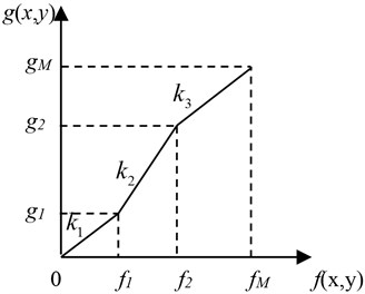
In the process of the image, a form of linear gray level transform can be used to highlight the image details in some gray levels and to properly lose some image details in the other gray levels. This linear gray level transform is called the piecewise linear transformation. Its expression is:

where $f_1$, $f_2$ is the gray value in original image. $f_M$ is the maximum gray value in original image. $g_1$, $g_2$ is the gray value in output image. $g_M$ is the maximum gray value in output image.

The curve of the piecewise linear function based on gray level transformation is shown in Fig. 2.

Fig. 2Gray level transformation contrast enhancement function

4. Using Shannon wavelet to get the time of arrival of signals

The time of arrival of the Lamb wave need to be accurately calculated in the process of the damage identification based on phased array theory. There are several time-frequency domain signal procession methods to calculate the time of arrival of the signals, such as, Hilbert Huang transform (HHT), Morlet wavelet transform, and so on. But HHT is restricted by decomposition and termination condition. Morlet wavelet may bring error in calculating the time of arrival to approximate value. In general, it is good solution to calculate the Lamb wave time of arrival by wavelet analysis because of its high time-frequency resolution. Shannon wavelet transform is presented to calculate the time of arrival of the Lamb wave in the following.

5. Experimental research

5.1. Experimental system

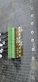
Experiments were conducted on a carbon fiber composite wing box of an unmanned aerial vehicle (UAV) to verify the theoretical results. The experimental setup is an integrated multi-channel PZT array scanning system. It has many functions, such as waveform generation, data acquisition, I/O control, magnification control, signal graphic display, waveform analysis and feature extraction, et al. The details are described in reference [26].

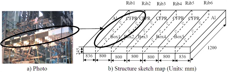
The main material of the wing box is carbon fiber-reinforced polymers (CFRP). The upper and lower boards are interlayer plates and their fabricated modes are: [45/0/-45/90/0/-45/0/90/-45/0/45/0]. Each interlayer is 0.16 mm thick. The upper and lower board is 3.68 mm thick. Fig. 3 gives the photo and the size of the box. The dimension of the wing box is 4000 mm×1200 mm×245 mm. A fixed side and a free side made of aluminum material are placed on the two sides of the wing box. Six ribs named Rib1, Rib2, Rib3, Rib4, Rib5 and Rib6 are placed in the wing box which is divided into five wing boxes called Box1, Box2, Box3, Box4 and Box5. The experiment is done in Box1. A PZT array is stuck in the middle of the structure. The PZT array consists of 9 PZT wafers arranged in a linear array with spacing at 2 mm. The diameter of the PZT wafer is 8 mm and the thickness is 0.2 mm.

Fig. 3Experiment specimen

5.2. Excitation signal central frequency selection

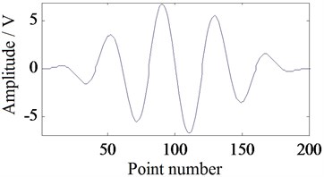
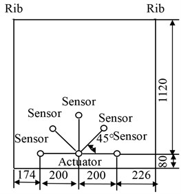
In order to get the central frequency of the excitation signal used in the experiment, the response signal generated by the excitation signal with the frequency from 30 KHz to 100 KHz is analyzed. The excitation signal waveform is shown in Fig. 4. The amplitude of the signal is 7 V. The number of wave peak is 5. Fig. 5 is the experimental specimen and the sensors array arranged in the structure. PZT sensors array are arranged in the direction of 0°, 45°, 90°, 135°, and 180°. The actuator and sensor in 90° are used in this experiment for signal central frequency selection. The distance between the actuator and the sensor is 200 mm. The central frequency of the excitation signal is selected according to simplicity of the Lamb wave mode. Fig. 6 is the response signal travelling in the structure with the central frequency from 30 KHz to 100 KHz. From Fig. 6 we can find, the mode aliasing is existed in the signal with the central frequency from 50 KHz to 100 KHz. Comparing the signal of 30 KHz central frequency with the signal of 40 KHz central frequency, the simplicity of the signal with 30 KHz central frequency is better. Therefore, 30 KHz central frequency is selected for the excitation signal in following experiments to excite A0 mode Lamb wave travelling in the structure.

Fig. 4Excitation signal

5.3. A0 mode Lamb wave speed measurement

Because the anisotropy of the carbon fiber composite, the wave speeds in all directions are different. In the experiment of the A0 mode Lamb wave group speeds of all directions travelling in the composite structure, the sensors array in the structure is arranged as Fig. 5. PZT sensors in the array are arranged in the direction of 0°, 45°, 90°, 135°, and 180°. The distance between the actuator and the sensor is 200 mm. The excitation signal waveform is shown in Fig. 4 .The central frequency of the signal is 30 KHz. The time of arrival of the excitation signal that calculated by Shannon wavelet is 0.2610 ms. The experimental sampling frequency $f_s$ is 2 MHz.

The times of arrival of the sensor signal that are calculated by Shannon wavelet in the direction of 0°, 45°, 90°, 135°, and 180° are 0.4455 ms, 0.4550 ms, 0.4755 ms, 0.4615 ms, and 0.432 ms respectively. The traveling times compared with excitation signals are 0.1845 ms, 0.1940 ms, 0.2145 ms, 0.2005 ms, and 0.1710 ms respectively. Therefore, the Lamb wave group speeds in the above five angle are 1084 m/s, 1030.9 m/s, 932.4 m/s, 997.5 m/s, and 1169.6 m/s respectively. The values of group speed in 0°-180° range (Fig. 6) are achieved by interpolation of quadratic polynomial in Matlab according to the 5 calculated A0 mode Lamb wave group speed values. The group speed values are used in the following process.

Fig. 5Sensor array for A0 mode Lamb wave group speed measurement

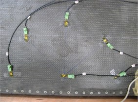
a) Photo of specimen

b) The structure sketch map (Units:mm)

Fig. 6The response signals travelling in the structure with the central frequency from 30 KHz to 100 KHz

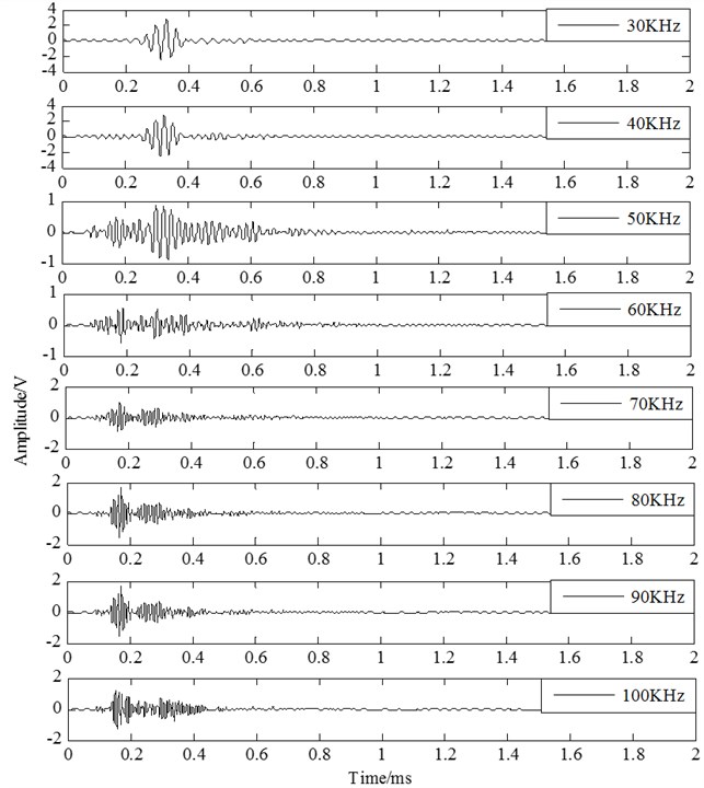
Fig. 7A0 mode Lamb wave group speed in a certain range

5.4. Damage identification experiment verification and analysis

5.4.1. Experiment with a PZT sensor array

The arrangement of the PZT array on the structure is presented as Fig. 8. The digital tags of 9 PZT wafers from left to right are [0, 1, 2,…, 8]. The marker of $Ф$30 mm round in the Fig. 8 is the position of the 0.2 kg weight load. The weight load is used to simulate the damage type of composite delamination. Because they are similar in causing Lamb wave scatting. And using weight load simulating damage can both ensure the experimental validity and spare experiment cost. The coordinate system origin is set to be the middle point of the array and the 0° direction coincides with the alignment of the array. The center coordinate of the load is (70°, 125 mm).

Fig. 8Arrangement of the PZT array

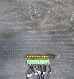
a) Photo of specimen

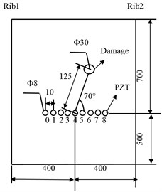
b) Structure sketch map (Units: mm)

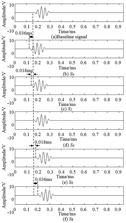
The excitation signal used in this experiment is shown in Fig. 9. The excitation signal emitted by each drive sensor is calculated by adding the time delay to the reference signal. The time delay is calculated by the Eq. (4). The number of the excitation signals is too much so that only one group data is given as example. Fig. 9 gives the reference signal and the excitation signals in angle 0° which the sensor 0, sensor 2, sensor 4, sensor 6, and sensor 8 act as actuator. Fig. 9(a) is the reference signal. The time of arrival calculated by Shannon wavelet is 0.237 ms. The figures from Fig. 9(b) to Fig. 9(f) are the excitation signals $S_0$, $S_2$, $S_4$, $S_6$ and $S_8$. Their time-delays are $\mathrm{\Delta }{t}_0\left(0^{\mathrm{o}}\right)=\text{–0.038 ms,}$$\mathrm{\Delta }{t}_2\left(0^{\mathrm{o}}\right)=-\text{0.019 ms,}$$\mathrm{\Delta }{t}_4\left(0^{\mathrm{o}}\right)=\mathrm{}\text{0 ms,}$$\mathrm{\Delta }{t}_6\left(0^{\mathrm{o}}\right)=\text{0.019 ms,}$$\mathrm{\Delta }{t}_8\left(0^{\mathrm{o}}\right)=\mathrm{}$0.038 ms. The minus in the time delay results represents that the signal is moved to the left. The experimental sample frequency $f_s$ is 1.6 MHz.

The process of experiment is as follows:

Firstly, data acquisition is carried out through the interval 0° to 180° to get the sensing signals collected in structural health state and in structural damage state respectively. The sensing signal collected in structural health state is named health signal and the sensing signal collected in structural damage state is named damage signal. The health signal is acted as a reference signal and the damage signal is compared with the reference signal to get the damage scattered signal in each direction. The health signal, damage signal and scattered signal collected from channel 2-1 in the experiment is shown in Fig. 10.

Fig. 9Excitation signal when PZT 0, 2, 4, 6 is actuator in angle 0

Secondly, the specific time delay $\mathrm{\Delta }{t}_i\left(\theta \right)$ is added to the damage scattered signal. This process is similar to the process that the time delay is added to the excitation signals. And the synthetic signal is got by cumulating all these signals in the same direction.

Thirdly, the amplitude of the synthetic signal is compared with the max amplitude of all signals to get its relative amplitude. The angle where the signal of the max amplitude lies in is the polar angle of the damage and the pole diameter of the damage is calculated from the signal that damage lies in. Fig. 11 is the normalized amplitude of the synthetic signals in each angle.

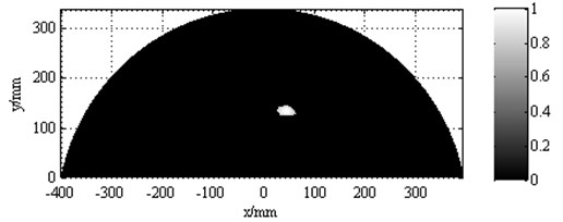
Finally, the normalized amplitude of synthetic signals is described on distance-direction two-dimensional plane in the gray form to get a mapped image. The synthetic signals in each angle from 0° to 180° are drawn on the mapped image. The location in the mapped image of the synthetic signal is calculated by the Eq. (9) and Eq. (10).The mapped image of damage identification is shown in Fig. 12. The monitoring scope is not a semicircle, because the experimental specimen is anisotropic CFRP. That is to say, in every direction, the signal collection points are equal but the Lamb wave group speed in different direction is different. Therefore the monitoring distance of the signal in each angle is different. The location of identification damage is (72°, 139.5). The location of the actual damage is (70°, 125 mm). Their angle error is 2° and the distance error of two points between identification damage and actual damage is 15.2 mm. The A0 mode Lamb wave group speed in the angle 72° is 962.4 m/s.

Fig. 10The health signal, damage signal and scattered signal collected from channel 2-1

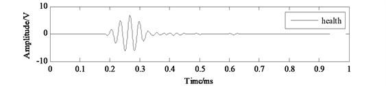
a) Health signal

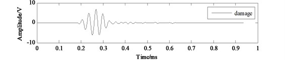
b) Damage signal

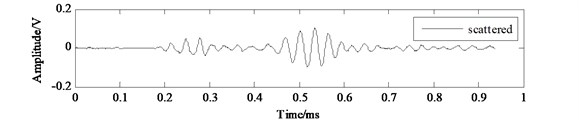
c) Scattered signal

Fig. 11Normalized signal of the synthetic signals in each angle

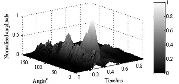
Fig. 12Mapped image of identification result

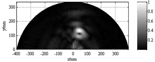
Fig. 13Contrast enhancement image

The identifiable degree of Fig. 12 is low. Gray transform method is applied to highlight the image. In the piecewise linear function Eq. (12) and Eq. (13), the parameters are $f_1=\text{0.1}$, $g_1=\text{0.05,}$$k_1=\text{0.5,}$$f_2=\text{0.7,}$$g_2=\text{0.1,}$$k_2=\text{1}/\text{12}\text{,}$$f_M=\text{1,}$$g_M=\text{1,}$$k_3=\text{3.}$ These parameters are put in the piecewise linear function to get the contrast enhancement imaging. The processed mapped image is shown in Fig. 13.

5.4.2. Screw loosening monitoring

Screw loosening monitoring experiment is done on CFRP wing box of an UAV. The phased array theory is utilized to identify the loose screw. The experiment specimen is present in Fig. 14. The digital tags of 9 PZT wafers from up to down are [0, 1, 2,…, 8]. The coordinate system origin is set to be the middle point of the array and the 0° direction ($x$ direction) coincides with the alignment of the array. The mark symbols of five screws from top to bottom are ①-⑤. The No.③ screw is loosening. The polar coordinates of the No.③ screw are (91.0°, 50.8 mm) and the polar coordinates of the No.④ screw are (73.3°, 52.2 mm).

Fig. 14Arrangement of the PZT array

a) Photo of specimen

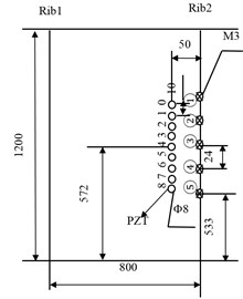
b) The structure sketch map (Units: mm)

Fig. 15Mapped image

Data acquisition is carried out on structural health state and structural damage state and the specific time delay $\mathrm{\Delta }{t}_i\left(\theta \right)$ is added to each signal in its emission and receiving process. The damage signal is compared with the health signal to get the damage scattered signal in each direction. All the damage scattered signals in the same direction are cumulated to get the synthetic signals. The normalized amplitude of the synthetic signals is drawn on a 2-D plane in a gray scale form to create a mapped image. In the piecewise linear function Eq. (12) and Eq. (13), the parameters are $f_1=\text{0.1,}$$g_1=\text{0.05,}$$k_1=\text{0.5,}$$f_2=\text{0.7,}$$g_2=\text{0.1,}$$k_2=\text{1}/\text{12}\text{,}$$f_M=\text{1,}$$g_M=\text{1,}$$k_3=\text{3}$. These are utilized in the original image to enhance the image identifiable degree.

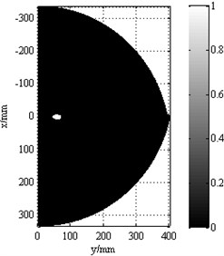
The phased array theory based structural health monitoring identification result processed by gray level transformation is shown in Fig. 15. The monitoring distance of the signal in each angle is different, because the Lamb wave group speed in each direction is different. The recognized location is (88°, 56.8). The locations of No.③ screw and No.④ screw are (91.0°, 50.8 mm) and (73.3°, 52.2 mm) respectively. Comparing the recognized location with the location of No. screw and the location of No.④ screw, the damage identification location is closer to No.③ screw. The angle error between the identification location and the location of No.③ screw is 3° and their distance error is 6.6 mm. In this case, loose screw can be identified on the No.③ screw. The A0 mode Lamb wave group speed in angle 88° is 1137.1 m/s.

6. Conclusions

The phased array theory based structural health monitoring for carbon composite wing box is researched. This method controls the beam steering by controlling the time delay of the emission signals and the receiving signals to scan the structure in a certain range automatically. The Shannon wavelet is utilized to calculate the time of arrival of the signals. The experiments using PZT linear sensors array in carbon composite structure to detect the damage and the screw loosening in the structure exemplify that the phased array theory well utilized in scanning damage in the structure and the gray level transformation based contrast enhancement damage image can clearly describe the damage in the structure.