Gearbox fault diagnosis based on local mean decomposition, permutation entropy and extreme learning machine

3.1. Definition of permutation entropy

Permutation entropy was firstly introduced by Bandit to estimate the complexity of time series through comparing the neighboring values [19]. The algorithm of PE can be described as follows:

Given a time series $\left\{x\left(k\right),k=\mathrm{1,2},\dots ,N\right\}$, the $m$ dimensional vector at time $i$ can be defined as:

where $m$ represents the embedding vector and $\tau$ represents time delay.

$x_i^m$ has a permutation ${\pi }_{r_0{r}_1\cdots r_{m-1}}$ if it satisfies:

where $0\le r_i\le m-1$ and $r_i\ne r_j$.

Aim at a $m$-tuple vector, there are $m!$ permutations. We define the relative frequency for each permutation as:

where $\mathrm{N}\mathrm{u}\mathrm{m}\mathrm{b}\mathrm{e}\mathrm{r}\left(x_i^m\right)$ is the number of satisfying the type $\pi$.

PE with $m$ dimension can be determined by:

It is easy to find that the maximum value of $H_{PE}$ is $\mathrm{I}\mathrm{n}(m!)$. So the normalized permutation entropy is:

It is obvious that $H_{PE}$satisfies ${\text{0}\le H}_{PE}\le \text{1}$. A larger value of $H_{PE}$ means the time series is much more irregular. When the time series is white noise, $H_{PE}$ obtains the maximum value (one). On the contrary, $H_{PE}$ with the smaller value is more periodic and the minimum value is zero. Therefore, PE is used to estimate the complexity and dynamic change of a signal.

3.2. The parameter selection of permutation entropy

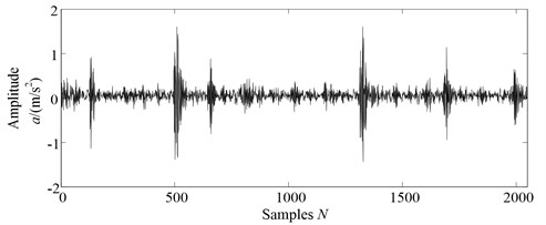
These parameters should be set before using PE, including embedding dimension $m$, time delay $\tau$ and the length of the time series $N$. In order to investigate the effect of each parameter in calculating PE value, an actual gearbox vibration signal is taken as the analyzed time series, which is shown in Fig. 1. Firstly, we conduct the research on the relationships between the PE values and length of the data $N$. Fig. 2 illustrates the PE values calculated by using the different data length $N$ and embedding dimension $m$, where the data lengths $N=$128, 256, 512, 1024, 2048 are respectively computed under the embedding dimension $m=$2-10. As can be seen from Fig. 2, when the data length is more than 512, the difference between the PE values with different data length $N$ is small. For example, when $m=$6, the difference between PE value with 512 points and PE value with 2048 points is only 0.0420. Hence, when $m=$6, the data length with more than 512 points is sufficient to obtain stable PE values.

Fig. 1The waveforms of vibration signal measured from gearbox experiment system

Secondly, the relationship between the PE values and time delay $\tau$ is investigated under the different dimension $m$. Fig. 3 shows the PE values computed with different time delay $\tau$ and embedding dimension $m\text{,}$ where $\tau =$1-6 are selected to achieve the PE values under the dimension $m=$2-10. The conclusion can be drawn from Fig. 3 that the time delay $\tau$ has little impact on the estimation of PE. For example, when $m=$6, the difference of PE values between $\tau =$1 and $\tau =$6 is only 0.0085. Therefore, in this paper, we select time delay $\tau =$1 in the following research.

Finally, the PE value highly depends on the selection of embedding dimension $m$. Bandt and Pompe [19] proposed the permutation entropy method and indicated that the method works with the embedding dimension 3$\le m\le$7. In addition, Cao et al. [20] have discussed the validity of permutation entropy under different conditions of embedding dimension. Obviously, when embedding dimension $m$ is too small, the scheme will not work since there are too few distinct states. On the other hand, when embedding dimension is too large, it will lead to time consuming [21]. Embedding dimension $m$ is often selected by considering between information loss and computational complexity, $m$ is set to 6 in this paper.

Fig. 2The PE values of gearbox signals with different lengths

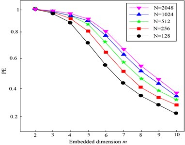
Fig. 3The PE values of gearbox signals with different time delays

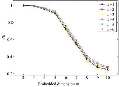
Fig. 4The MPE values of gearbox signals with different embedding dimensions

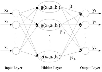
Fig. 5The structure of ELM

5.1. The fault feature extraction based on LMD, PE and SVM

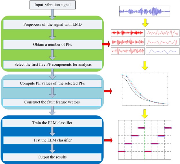
LMD has advantages in end effect and less mixing phenomenon compared with EMD, which can result in better decomposition results. The advantages of LMD has been verified by reference [26]. After a series of PFs are obtained using the LMD, the PE values of PFs (called PF-PE) are extracted as the feature vectors for fault type identification, compared with approximate entropy (ApEn) [8] and sample entropy (SE) [9], Permutation entropy (PE) are simple, fast and immune to noise. Lastly, ELM has been proved to require less human intervention and less running time than support vector machine (SVM) [18]. So in this paper, ELM is introduced for identification and classification of gear under different conditions. Based on the superiorities of LMD, PE and ELM, a novel gear fault diagnosis approach is proposed in this paper, the detailed steps can be summarized as follows:

1) When the gearbox under different working conditions, the vibration signals are acquired by acceleration sensors at a sampling frequency $f_s$.

2) Partition the measured vibration signal into non-overlapping windows of suitable size $N$.

3) Apply LMD method to analyze the measured vibration signal, and a number of PF components can be obtained. Then, the first five PF components that contain the most fault information are selected for further analysis.

4) Calculate PE values of the selected PF components using Eqs. (11)-(15) and generate the feature vector. Note that the obtained PE values of PF components are called PF-PE and the parameters of PE are set as follows: data length $N=$2048, $m=$6 and time delay $\tau =$1.

5) The obtained fault features are fed into fault classifier ELM for training and testing to fulfill the fault diagnosis automatically. Note that the number of hidden neurons is assigned to 80 and sigmoid function is selected as the activation function in this paper.

A functional framework based on PF-PE and ELM algorithm is presented in Fig. 6.

Fig. 6Flowchart of the proposed algorithm

5.2. Experimental data analysis

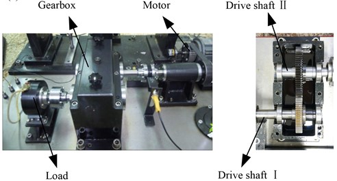
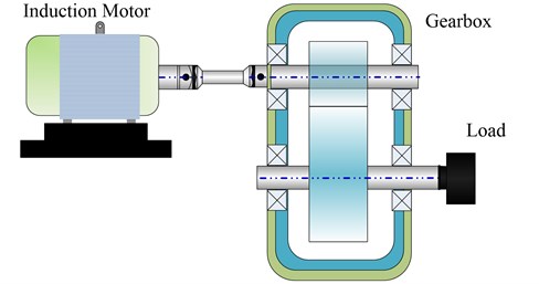
To illustrate the effectiveness of the proposed methodology in the real applications, experimental analysis on gear with slight wearing, severe wearing and missing tooth are conducted. The experiment is conducted on a test rig of the transmission gearbox, the layout and schematic sketch of the fault experiment platform are shown in Fig. 7(a) and (b), respectively. Two High Sensitivity Quartz ICP accelerometers were installed for data acquisition (one vertical, and one horizontal), the location of the accelerometer is on the base of floor stand. The speed of the motor is set to be 1500 rpm. Meanwhile, the sample frequency is 10000 Hz and the sampling time is 1 s. The fault gear is installed on the driven gear and the working parameter of the gearbox is listed in Table 1. Four working conditions are considered in this experiment: normal, slight wearing tooth, severe wearing tooth and the missing tooth. The wearing gear with different severities and gear with missing tooth are shown in Fig. 8, respectively.

Fig. 7The layout and schematic sketch of the fault experiment platform

a)

b)

Fig. 8The input fault position of gears

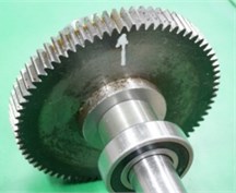
a) Slight wearing

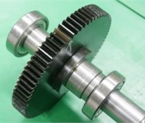
b) Severe wearing

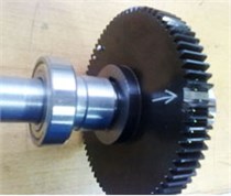
c) Missing tooth

Since the gear fault vibration is a multi-component, amplitude-modulated and frequency-modulated signal, the LMD method can decompose a complicated signal into a serial of PFs adaptively. So the LMD method is especially suitable for processing the gear fault signal. Firstly, the LMD method is applied to decompose the signal into a number of PFs, and then the PE values of the first five PFs are computed to construct the feature vectors. Finally, ELM is used to recognize the various fault types of gearbox [21].

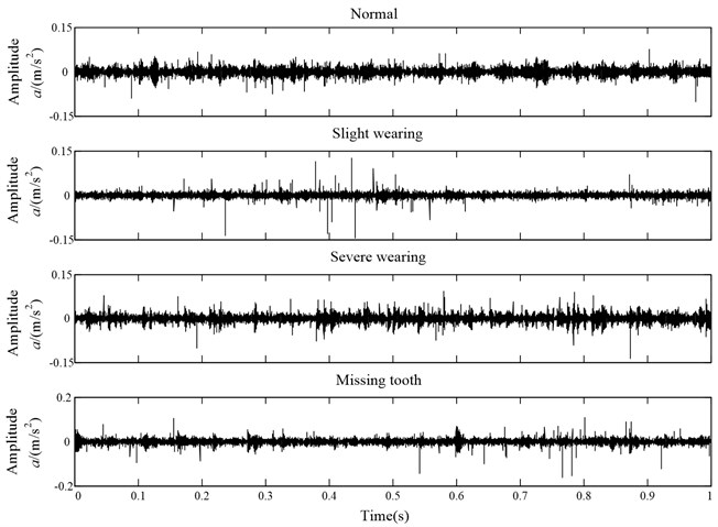
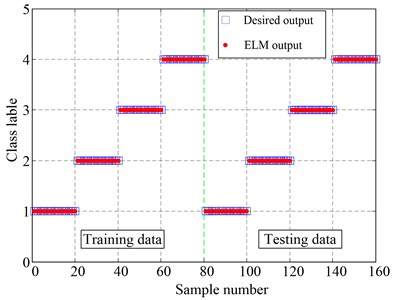
In this experiment, the collected vibration signals consist of four working conditions. Actually, the experimental analysis is a four-class recognition problem. The vibration signals are divided into several non-overlapping segments with the length $N=$2048. Each condition has 40 samples, and there are total 160 samples, in which 80 samples will be randomly selected as the training data, while the remaining 80 samples are used to test the ELM classifier. The detailed numbers of samples description for each bearing condition are shown in Table 2. The time domain waveforms of vibration signals under four fault categories case are depicted in Fig. 9, respectively.

Fig. 9The waveforms of gearbox vibration signal under four different conditions

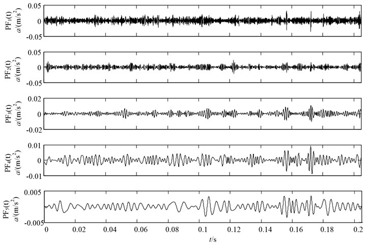
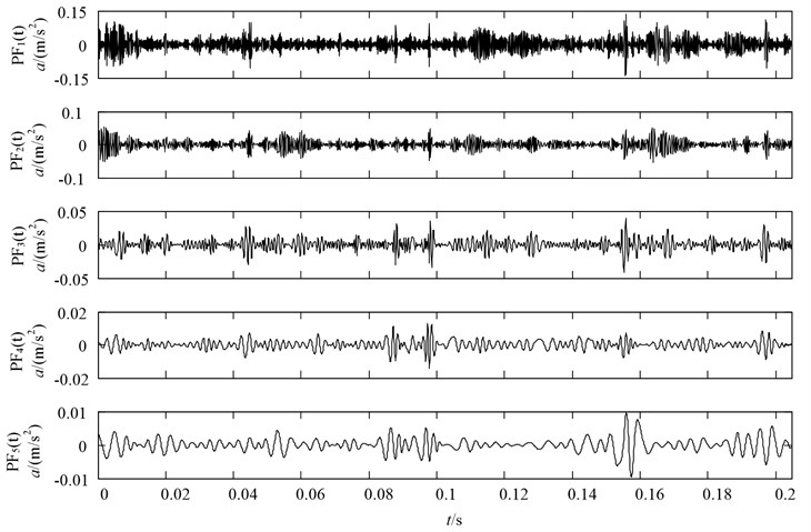
Since the measured vibration signal has the characteristics of nonlinear and non-stationary, LMD is applied to decompose the vibration signal into a series of PFs. The decomposition results with four conditions (including: normal state, slight wearing fault, severe wearing fault and missing tooth fault) are illustrated in Figs. 10-13, respectively. Note that since the fault information contains mainly in the front PF components, only the first five PF components are plotted for saving space.

After completing the decomposition using LMD method, the PE method is utilized to extract the fault features according to the flowchart of the LMD and PE algorithm, which are described in Section 5. In this paper, the parameters of PE are set as follows: embedding dimension $m=$6, time delay $\tau =$1. To illustrate the advantage of the PF-PE for fault feature extraction, the PE values of the original vibration signals are also calculated for comparison. The PE values of different working conditions (including normal condition, slight wearing fault condition, severe wearing fault condition and missing tooth fault condition) are shown in Fig. 14. It should be noted that scale value 0 in the horizontal axis corresponds to the PE value of original signal and the scale values 1-10 in the horizontal axis correspond to the values of the first PF-PE value to the tenth PF-PE value [25].

Fig. 10LMD decomposition results of the vibration acceleration of gear with normal condition

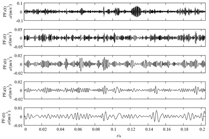
Fig. 11LMD decomposition results of the vibration acceleration of gear with slight wearing fault condition

As seen from Fig. 14, the following conclusions can be got: Firstly, it can be observed from the PE of original signal (scale value 0) that PE can describe the gearbox under different working conditions. However, the PE values of fault conditions are too close to recognize them effectively.

Fig. 12LMD decomposition results of the vibration acceleration of gear with severe wearing condition

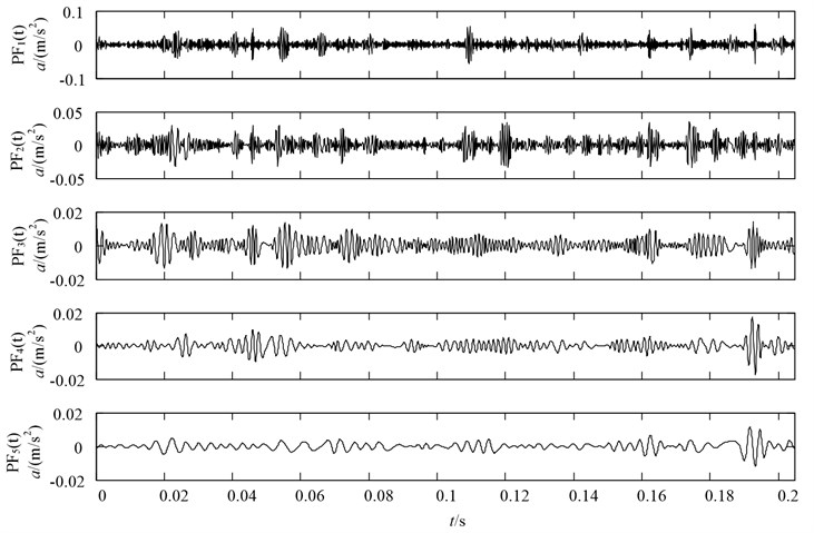
Fig. 13LMD decomposition results of the vibration acceleration of gear with missing tooth condition

This implies the complexities of signals under the above three fault conditions are similar and the simply performing the PE of original signal cannot distinguish them effectively. Therefore, there remains a need for a denoising method to enhance the fault characteristics. Secondly, PF-PE values of fault working conditions are all higher than that of normal conditions. It is because that when the gearbox operates with local defect, it would appear periodical impulses with high frequency, hence, the complex degree of PF-PE values will increase. Thirdly, although the gearbox with different working conditions has different PF-PE values, they represent the similar trend, which consists well with real working condition of gearbox. Lastly, it can be observed from Fig. 14 that the front five PF-PE values exhibit higher distinguishability than the others, it is the reason that the front five PFs contains the main fault information.

Apparently, in this experiment, the front five features with most important information of the vibration signal are selected to form the new feature vectors. Naturally, the new feature vectors are used to train the ELM and then the test data set is applied to validate the recognition accuracy of ELM. According to the description in Table 2, 80 samples are randomly selected as training data, and the residual 80 samples are taken as testing data.

The experiment is repeated 10 times and the average classification results of the proposed method are shown in Fig. 15, which include the ELM outputs and the desired outputs about the training and testing samples. As can be seen, there are no training and testing samples misclassified and the average recognition accuracy reaches to 100 %. The comparison results demonstrate that the new proposed approach performs a good classification result, which is exactly suitable and effective in gear fault diagnosis.

Fig. 14Comparisons of PE and PF-PE of gearbox with different working conditions

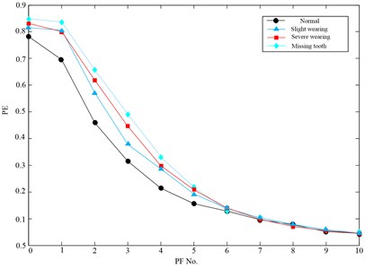
Fig. 15Classification results of the proposed method

For comparison purpose, the sample entropy (SE) method is also used to analyze the gear data [9], and the fault features obtained by PF-SE are also fed into ELM for pattern identification. Note that only the first five PFs are selected to calculate the SE values for comparison. Through the same process which includes the number of training and testing samples and the parameter selection of ELM, the classification results based on PF-SE and ELM are shown in Table 3. It can be easily found that one sample with slight wearing, one sample with severe wearing fault as well as three samples with missing tooth fault are misclassified. The total testing classification accuracy is 93.75 %, while the testing classification accuracy of PF-PE is 100 %. The comparisons demonstrate the fault features extracted using PF-PE method can better describe the characteristics of vibration signal, which has higher reparability than that of PF-SE method. Thus, PF-PE has a prominent advantage over PF-SE in terms of feature extraction under variable conditions of gearbox.

Back Propagation (BP) and support vector machine (SVM) are widely used in the classification, so a comparison among ELM, SVM and BP is conducted to validate the advantages of ELM. Besides, the training and testing data are the same in each algorithm. The classification accuracy and consuming time of each classifier using PF-PE as feature extractor are summarized in Table 4.

Through comparing the classification results, we can draw the conclusions that ELM has the highest accuracy and the least consuming time among three classifiers, it reinforces the superiority of the ELM in classification performance. Moreover, the comparison results show that the proposed PF-PE combined with ELM has outstanding performance in fault diagnosis of gearbox, which can be applied to recognize the different categories of gears.

In order to illustrate the potential application of proposed methodology, a comparative study between the present work and published literature presented in Table 5 [5, 26-29]. The comparing items include the machine elements used, fault severity levels, feature extraction method and classifier used, classified states, maximum classification efficiencies and denoising technique.