An improved longitudinal vibration model and dynamic characteristic of sucker rod string

1. Introduction

The sucker rod pumping system is one of the mechanical recovery methods in the world’s oil industry and it is by far the predominant artificial lift method used in the world for producing oil well [1-3]. And SRS is a slender rod of several kilometers, which transmits the movement from mechanical rotary motion to plunger linear motion. Meanwhile, the characteristic analysis of SRS’s longitudinal vibration is foundation of system fault diagnosis and oil production forecast. Therefore, the dynamic simulation of SRS draws more and more attention from domestic and foreign scholars. One of the most relevant and successful simulation model describing the sucker rod dynamics is developed by Gibbs [4], then Gibbs [5-8] extends SRS dynamics to computer-based diagnostics of the down-hole well conditions. An improved model of SRPS is built by Dale Russel Doty and Zelimir Schmidt et al. [9], incorporating the dynamics of the liquid columns as well as SRS through a system of partial differential equations. Subsequently, based on the improved model, the dynamic simulation of SRPS is carried out by S. D. L. Lekia and H. A. Tripp et al., and the model is verified by comparing it with the experimental data [10-12]. Then Lukasiewicz, S. A. and J. Xu, et al. [13, 14] apply the dynamic simulation technique of SRPS to a slant-hole or horizontal well, and build a longitudinal vibration model of SRS in a horizontal well. Recently, DaCunha, I. N. Shardakov and Luan Guo-hua [1, 3, 15] analyse boundary conditions effecting rod law of motion and correct the excitation forces of rod longitudinal vibration. In the detail, The SRS’s longitudinal vibration is described with the semi-infinite-spatial-domain wave equation by DaCunha. Shardakov thinks that the multivalued force-velocity relation arises due to the operation of pump valves and Coulomb’s friction, the numerical model of SRS’s longitudinal vibration is built. A new one-dimensional vibration model of SRS for deep well is built by G. H. Luan, considering the structure of the improved side-flow pump.

However, the most of aforementioned approaches have not been studied sufficiently. In the detail, the empirical formula or simplified formula is usually used to build the simulation model of plunger load [16-18]. Obviously, it is hardly possible for empirical formula to meet the precision requirement of plunger load. And the simplified formula is obtained based on the specific oil wells, which does not suit the other wells. For example, there are two methods for computing the friction of pump plunger. The experiment is carried out with water instead of lubricant [19], and the empirical formula is given [17, 19, 20], as follows:

where, $F_{pf}$ is the liquid friction of pump plunger (N); $D_p$ is the diameter of pump plunger (mm); $\delta$ is the gap between pump plunger and pump barrel (mm).

The Eq. (1) was given under some assumptions by Wan B. J. [19]. Wan thought that the produced fluid in oil-water was the unstable emulsion when the oil well had high water content such as more than 50 %. In the oil well, the liquid was easily layered into crude oil and water, the crude oil was dispersed phase and the water is continuous phase. Therefore, Wan thought that the liquid was mainly water between pump plunger and pump barrel. Based on the above analysis, the lubricant of half dry friction of plunger could be replaced with water [19].

As a result, the above formula is obtained under the high water content condition, which only applies to the water-flood or thin oil well. However, when the oil well is a polymer flooding or heavy oil well, the liquid of oil well is Non-Newtonian power law fluid, the Eq. (1) will be inappropriate.

With the second method, the liquid is used as Newtonian power law fluid, and the liquid friction of pump plunger is derived based on gap flow theory of hydromechanics [20], as follows:

where, $\mu$ is the instantaneous dynamic viscosity of liquid, kg/(s∙m); $v_p$ is the velocity of pump plunger (m/s); $L_p$ is the length of pump plunger (m); $\mathrm{\Delta }P$ is the pressure difference inside and outside of pump (Pa); $\epsilon$ is the eccentric distance (m).

The Eq. (2) was derived in ideal circumstances [20]. For example, the inner surface of pump barrel as well as the outer surface of pump plunger is defined as an ideal cylindrical surface. However, those surfaces are not absolute straight cylindrical surfaces, and the crevices of the surface are not formed by ideal parallel surfaces. In addition, the Eq. (2) is derived under the Newtonian fluid, which will not apply to the oil well of non-Newtonian power law fluid. According to the above analysis, the computing model of plunger friction needs to be derived for the oil well of non-Newtonian power law fluid.

The current simulation models of plunger load contain the model of hydraulic loss [21, 22] and the model of clearance leakage [23, 24], the formulas are as follows:

where, ${\rho }_g$ is the gravity gradient of liquid (N/m³); $A_p$ is the cross-sectional area of pump plunger (m²); $A_v$ is the area of valve’s aperture (m²); $\gamma$ is the flow coefficient.

From Eq. (3), the hydraulic loss of pump is proportional with the speed squared of pump plunger. However, in order to obtain linear solution, the formula of hydraulic loss is usually linearized at present. Generally, the speed of pump plunger is defined as constant with stroke number and frequency. Therefore, the simulation result will not reflect the influence of the instantaneous speed of pump plunger on hydraulic loss of pump. With Eq. (4), the problem of annular pressure difference-shear leakage direction of pump is discussed, but the influence of the NNPLF on the annular pressure is not considered.

According to the analyses above, the simulation models of plunger nonlinear friction, hydraulic loss and clearance leakage need to be improved with the action of NNPLF. Considering the influence of the time-varying characteristics of some dynamic parameters on the plunger load, such as plunger nonlinear friction, hydraulic loss and clearance leakage, the simulation model of plunger load needs to be corrected. Finally, considering the influence of the nonlinear characteristics of plunger load and SRS friction on the SRS’s longitudinal vibration, the simulation model of SRS’s longitudinal vibration needs to be improved.

In this paper, in section 2, an improved simulation model of mix SRS with absorber is built. The computational model of pump plunger load is corrected. In the details, based on the flow characteristic of NNPLF, a new computational model of NNPLF’s velocity between pump plunger and pump barrel is established. Then the law of the velocity distribution is solved out with Lagrange multiplier method. Therefore, the nonlinear friction between NNPLF and SRS as well as the nonlinear friction between NNPLF and pump plunger is derived. Taking account of the influence of nonlinear characteristics of some parameters on the pump plunger load, such as plunger friction, hydraulic loss and clearance leakage, an improved model of the pump load is derived. In section 3, the dynamic response is solved out with fourth order Runge-Kutta method. In section 4, a wireless indicator is used to verify the feasibility of the proposed dynamics simulation method, and the sensitive parameters of plunger load and dynamic characteristic of mix SRS with absorber are analyzed. In section 5, the signification of dynamic simulation research on SRS and the conclusions are summarized.

2. The dynamic simulation model of SRS’s longitudinal vibration

The number stages of SRS assemblage are supposed to be $k$, and the polished rod displacement is $u^{*}\text{.}$ The relative displacement between polished rod and SRS top is $u_0$. Considering the influence of some factors on the SRS longitudinal vibration, such as SRS absorber between polished rod and SRS top, nonlinear friction between SRS and NNPLF and nonlinear plunger load, a mechanical model of SRS’s longitudinal vibration is established, as shown in Fig. 1.

Fig. 1The mechanical model of SRS’s longitudinal vibration

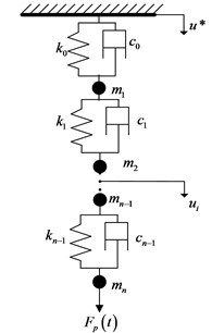
Based on the mechanical model of longitudinal vibration, a mathematical model is built, as follows:

where:

When $\left\{u\right\}={\left\{u_1,u_2,\dots ,u_{n-1},u_n\right\}}^T$, the equation is obtained as follows:

where, $c_i$ is the friction coefficient (Pa.s); $F_p$ is the load of pump plunger (N); $k_i$ is the stiffness coefficient of the $i$th element, m²; $C_i$ is the damping coefficient of the $i$th element, Pa; $u_i$ is the displacement of the $i$th element, m. $P_p\left(t\right)$ is the liquid load of pump plunger (kN); $F_{pf}$ is the friction between pump plunger and pump barrel (kN).

2.1. The nonlinear friction of pump plunger and clearance leakage

A structure schematic of pump plunger and pump barrel is given in Fig. 2. $L_p$ is the length of pump plunger, $R_p$ is the radius of pump plunger, $R_{pb}$ is the radius of pump barrel, $\delta$ is the gap between pump plunger and pump barrel.

Fig. 2The structure schematic of pump plunger and pump barrel

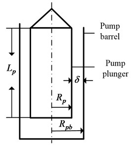
The liquid of oil well is supposed to be NNPLF with a homogeneous incompressible fluid and the oil well is a vertical well. The pump plunger and pump barrel are defined as rigid body with no elastic deformation and the pump barrel is static.

Based on the constitutive equation and shearing stress equation of NNPLF, the formula is given, as follows:

8

$\left\{\begin{array}{l}{\tau }_{pl}=K_{pl}{\left(\frac{d{v}_p}{dr}\right)}^n,\\ \frac{d}{dr}\left(r{\tau }_{pl}\right)=r\left(\frac{dp}{dz}\right).\end{array}\right.$

The radial velocity gradient of NNPLF between pump plunger and pump barrel is derived based on the above formula:

9

$\frac{d{v}_p}{dr}={\left[\frac{f}{2K_{pl}}\left(r+\frac{2C}{r}\right)\right]}^{\frac{1}{n}},$

where:

10

$f=\frac{\partial p}{\partial z},$

where, $C$ is the undetermined parameters; $n$ is the power law exponent; $k_{pl}$ is the consistency coefficient; $f$ is the axial pressure gradient of NNPLF in the annulus.

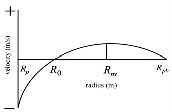
The velocity of NNPLF in annulus is influenced by pressure difference flow and pulsatile flow, the velocity distribution curve is given in Fig. 3. In Fig. 3, $R_0$ is the distance from a point with zero velocity of NNPLF to the centerline of pump plunger (m); $R_m$ is the distance from a point with maximum velocity of NNPLF to the centerline of pump plunger (m); $R_p$ is the radius of pump plunger (m); $R_{pb}$ is the radius of pump barrel (m).

Fig. 3The velocity distribution curve of NNPLF

When $r=R_m$ and $d{v}_p/d_r=$0, then:

11

$\frac{d{v}_p}{dr}={\left[\frac{f}{2K_{pl}}\left(r-\frac{R_m^2}{r}\right)\right]}^{\frac{1}{n}}.$

Therefore, the velocity distribution law of NNPLF and the boundary conditions are obtained:

12

$\left\{\begin{array}{l}v\left(r,t\right)={\int }_r^{R_{pb}}{\left[\frac{f}{2K_{pl}}\left(r-\frac{R_m^2}{r}\right)\right]}^{\frac{1}{n}}dr,\\ {\int }_{R_p}^{R_0}{\left[\frac{f}{2K_{pl}}\left(r-\frac{R_m^2}{r}\right)\right]}^{\frac{1}{n}}dr=\frac{d{u}_{pl}}{dt},\\ 2\pi {\int }_{R_p}^{R_{pb}}vrdr=\pi R_{pl}^2\frac{d{u}_{pl}}{dt},\\ {\int }_{R_0}^{R_m}{\left[\frac{f}{2K_{pl}}\left(r-\frac{R_m^2}{r}\right)\right]}^{\frac{1}{n}}dr={\int }_{R_m}^{R_{pb}}{\left[\frac{f}{2K_{pl}}\left(r-\frac{R_m^2}{r}\right)\right]}^{\frac{1}{n}}dr.\end{array}\right.$

The analytical formulas of the parameters are not derived, such as $R_0$, $R_m$, $f$. So the Lagrange multiplier method is used to find the numerical solution. Firstly, the variables are defined, as follow:

13

$\widehat{x}=\left[x_1\mathrm{}\mathrm{}\mathrm{}{x}_2\mathrm{}\mathrm{}\mathrm{}\mathrm{}{x}_3\right]=\left[R_{0\mathrm{}}\mathrm{}\mathrm{}\mathrm{}{R}_m\mathrm{}\mathrm{}\mathrm{}\mathrm{}f\right].$

Combining Eqs. (12) and (13), the constraint and the objective functions are derived:

14

$\left\{\begin{array}{l}\mathrm{m}\mathrm{i}\mathrm{n}F\left(\widehat{x}\right)=\left|{\int }_{R_p}^{R_{pb}}{\left[\frac{f}{2K_{pl}}\left(r-\frac{R_m^2}{r}\right)\right]}^{\frac{1}{n}}dr-v_{pl}\right|,\\ g\left(1\right)=R_{pb}-x_2\ge 0,\\ g\left(2\right)=x_2-x_1\ge 0,\\ g\left(3\right)=x_1-R_p\ge 0,\\ g\left(4\right)={\int }_{x_2}^{R_{pb}}{\left[\frac{x_3}{2K_{pl}}\left(r-\frac{x_2^2}{r}\right)\right]}^{\frac{1}{n}}dr\ge 0,\\ h\left(1\right)=2\pi {\int }_{R_p}^{R_{pb}}r{\int }_r^{R_{pb}}{\left[\frac{x_3}{2K_{pl}}\left(x-\frac{x_2^2}{x}\right)\right]}^{\frac{1}{n}}dxdr-\pi R_{pl}^2{v}_{pl}=0,\\ h\left(2\right)={\int }_{R_p}^{x_1}{\left[\frac{x_3}{2K_{pl}}\left(r-\frac{x_2^2}{r}\right)\right]}^{\frac{1}{n}}dr-v_{pl}=0,\\ h\left(3\right)={\int }_{x_1}^{x_2}{\left[\frac{x_3}{2K_{pl}}\left(r-\frac{x_2^2}{r}\right)\right]}^{\frac{1}{n}}dr-{\int }_{x_2}^{R_{pb}}{\left[\frac{x_3}{2K_{pl}}\left(r-\frac{x_2^2}{r}\right)\right]}^{\frac{1}{n}}dr=0.\end{array}\right.$

The parameters $R_0$, $R_m$, $f$ are solved out based the Lagrange multiplier method, and the velocity distribution law is expressed fully. Therefore, the friction of pump plunger is given as follows:

15

$F_{pf}=2\pi R_p{L}_p{K}_{pl}{\left({\left.\frac{d{v}_p}{dr}\right|}_{r=R_p}\right)}^n.$

Eq. (15) can be defined as follows:

16

$F_{pf}={\lambda }_{pl}{v}_p^n,$

where:

17

${\lambda }_{pl}=\frac{2\pi K_{pl}{L}_p\left(R_p^2-R_m^2\right)}{{\left[\underset{R_p}{\overset{R_0}{\int }}{\left(r-\frac{R_m^2}{r}\right)}^{\frac{1}{n}}dr\right]}^n},$

where, ${\lambda }_{pl}$ is the resistance coefficient of pump plunger, $\text{N}·{\left(\text{s}/\text{m}\right)}^n/\text{m}$.

The computing method of the nonlinear friction between SRS and NNPLF is the same as for the nonlinear friction between pump plunger and pump barrel, so we will not repeat it here.

Combining Eq. (11), the computing model of clearance leakage between pump plunger and pump plunger is derived, as follows:

18

$q_{vm}=\frac{\pi D_{p}n}{1+2n}{\left(\frac{\mathrm{\Delta }{p}_{io}}{k_{pl}{L}_p}\right)}^{\frac{1}{n}}\left[{\left(R_m-R_p\right)}^{\frac{1+2n}{n}}+\right.\left.\mathrm{}{\left(R_{pb}-R_m\right)}^{\frac{1+2n}{n}}\right]-\pi D_p{v}_p\left(R_m-R_p\right).$

Combining Eqs. (11) and (17), when $n=$ 1, $\mu =k_{pl}$, the equation of velocity of pump plunger is obtained, as follows:

19

$v_p=\frac{1}{2}\frac{\mathrm{\Delta }{p}_{io}}{\mu L_p}\left[{\left(R_m-R_p\right)}^2-{\left(R_{pb}-R_m\right)}^2\right].$

Combining Eqs. (18) and (19), when $n=$1, $\mu =k_{pl}$, $\delta =R_{pb}-R_p$, the computing model of clearance leakage of Newtonian fluid under laminar flow is derived:

20

$q_v=\frac{\pi {\delta }^3{D}_p\mathrm{\Delta }{p}_{io}}{12\mu L_p}-\frac{\pi \delta D_p{v}_p}{2}.$

When $\epsilon =$0, the Eq. (4) is the same as above Eq. (20).

2.2. The computational model of liquid load of pump plunger

Currently, the computational model of liquid load of pump plunger is given as follows:

21

$P_p\left(t\right)=A_p\left(p_d-p\right)-A_{Lr}{p}_d,$

where, $A_p$ is the cross area of pump plunger (m²), $A_{Lr}$ is the cross area of SRS bottom (m²), $p_d$ is the discharge pressure (Pa), $p$ is the instantaneous liquid pressure in pump (Pa).

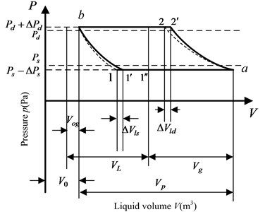
From Eq. (21), the instantaneous liquid pressure is a major factor which affects liquid load of pump plunger. The current model of instantaneous liquid pressure is built based on the Newtonian fluid. In this paper, a new model of instantaneous liquid pressure is built based on the NNPLF. The liquid pressure law in pump is given in Fig. 4 [25]. In Fig. 4, $V_x$ is the instantaneous volume of movement distance of pump plunger (m³), $V_p$ is the effective volume of movement distance of pump plunger (m³), $V_0$ is the clearance volume of pump (m³).

Fig. 4The liquid pressure law in pump

2.2.1. Liquid flowing into pump in the up stroke

When the standing valve is open, the liquid is drawn into the pump. At this point, the instantaneous liquid pressure of pump is influenced by the submergence pressure and the hydraulic loss. The formula of instantaneous liquid pressure is derived:

22

$P=P_s-\mathrm{\Delta }{P}_s,$

where:

23

$\mathrm{\Delta }{p}_i=n_v\rho \frac{1}{{\gamma }^2}{\left(\frac{d{u}_p}{dt}\right)}^2{\left(\frac{A_p}{A_v}\right)}^2\left(\frac{3n+1}{2n+1}\right)\left[\frac{n+3}{2\left(5n+1\right)}{\left(\frac{A_v}{A_p}\right)}^2-\left(\frac{A_v}{A_p}\right)+\frac{3\left(2n+1\right)}{2\left(5n+1\right)}\right],$
$i=s,d,$

where, $\mathrm{\Delta }{P}_s$ is the part hydraulic loss of standing valve (Pa); $u_p$ is the instantaneous displacement of pump plunger (m); $\rho$ is the density of liquid (kg/m³). $n_v$ is the number of traveling valve.

2.2.2. Fluid leaving pump in the down stroke

When the traveling valve is open, the liquid is discharged from the pump. At this point, the instantaneous liquid pressure of pump is influenced by the discharge pressure and the hydraulic loss. The formula of instantaneous liquid pressure is derived:

24

$P=P_d+\mathrm{\Delta }{P}_d,$

where, $\mathrm{\Delta }{P}_d$ is the part hydraulic loss of traveling valve (Pa), and the formula of hydraulic loss of traveling valve is Eq. (23).

2.2.3. Compressing phase of gas in the down stroke

When the standing valve is close and before the traveling valve is open, the pump plunger moves from top dead to down. Then the gas is compressed in the pump. Based on the polytropic process of gas, the formula of instantaneous liquid pressure is derived:

25

$p={\left[\frac{V_g}{V_g-V_p+V_x-\mathrm{\Delta }{V}_{ld}}\right]}^{n_q}\left(P_s-\mathrm{\Delta }{P}_s\right),$

where:

26

$\left\{\begin{array}{l}{V}_g=\frac{r_a}{1+r_a}\left(V_0+V_p\right),\\ V_x=A_p\left[u_p-\frac{A_p\mathrm{\Delta }P{L}_t}{E_t{A}_t}\right],\end{array}\right.$

where, $V_g$ is the volume of free gas in the pump (m³); $P_s$ is the submergence press of pump (Pa); $\mathrm{\Delta }{V}_l$ is the volume of clearance leakage between pump plunger and pump barrel (m³); $\mathrm{\Delta }P$ is the pressure difference between inner and outer pump (Pa); $r_a$ is the ratio of gas and liquid (m³/m³); $D_{pb}$ is the diameter of pump barrel (m); $\mu$ is the dynamic viscosity, kg/(s∙m); $L_p$ is the length of pump plunger (m); $u_p$ is the instantaneous displacement of pump plunger (m); $L_t$ is the length of tube (m); $E_t$ is the elasticity modulus of tube (N/m²); $A_t$ is the cross area of tube (m³).

When the traveling valve is opening, the time is defined as $t_{tv}$, the volume of movement distance of pump plunger is defined as $V_{tv}$, the volume of clearance leakage is defined as $\mathrm{\Delta }{V}_l\left(t_{tv}\right)$. The the equilibrium equation is obtained as follows:

27

$V_g-V_p+V_{tv}-\mathrm{\Delta }{V}_{ld}\left(t_{tv}\right)=V_g{\left(\frac{P_s-\mathrm{\Delta }{P}_s}{P_d+\mathrm{\Delta }{P}_d}\right)}^{\frac{1}{n_q}}.$

So, the gas of the clearance volume is derived as follows:

28

$V_{og}=\frac{V_0}{V_0+V_{tv}}\left[V_g-V_p+V_{tv}-\mathrm{\Delta }{V}_{ld}\left(t_{tv}\right)\right].$

2.2.4. Expanding phase of gas in the up stroke

When the traveling valve is close and before the standing valve is open, the pump plunger moves from bottom dead to up. Then the gas is expanded in the pump. With polytropic process of gas, the formula of instantaneous liquid pressure is derived:

29

$p={\left[\frac{V_{og}}{V_{og}+V_x-\mathrm{\Delta }{V}_{ls}}\right]}^{n_q}\left(P_d+\mathrm{\Delta }{P}_d\right).$

When the standing valve is opening, the time is defined as $t_{sv}$, the volume of movement distance of pump plunger is defined as $V_{sv}$, the volume of clearance leakage is defined as $\mathrm{\Delta }{V}_l\left(t_{sv}\right)$. Then the equilibrium equation is obtained as follows:

30

$V_{og}+V_{sv}-\mathrm{\Delta }{V}_{ls}\left(t_{sv}\right)=V_{og}{\left(\frac{P_d+\mathrm{\Delta }{P}_d}{P_s-\mathrm{\Delta }{P}_s}\right)}^{\frac{1}{n_q}}.$

3. The numerical model of SRS’s longitudinal vibration

The system equations of nonlinear longitudinal vibration of SRS are solved by fourth-order Runge-Kutta method, and the numerical model of longitudinal vibration of SRS is obtained. In this paper, the SRS is decomposed into five hundred elements, so the element length is four meters. Based on the basic parameters of beam pump system, the dynamic responses of system are obtained. Comparing the plunger displacements of two contiguous periods, if good agreement is found between the two simulation results within the allowed error range, the computing of the corresponding program will be stopped, and the dynamic response will be obtained:

where:

In addition, for the first calculation, the initial conditions are the same for all the plots as given below:

4. Experiment and discussion

The basic parameters are as follows: the well number is #62-39; the outdoor temperature during testing $T_{ho}$ is 28°C; the pumping unit type is YCYJ12-5-89HB; the motor type is YCCH250-8; the rated power of the motor with high rotating variation $P_H$ is 30 kW; the length of belt $L$ is 4 m; the linear density of single belt $\rho$ is 0.37 kg/m; the cross-sectional area of belt $A$ is 1.55×10^-4 m²; the coefficient of friction of the belt against the pulleys $\mu$ is 0.6; the diameter of the small pulley installed on the motor output shaft $D_1$ is 0.3 m; the diameter of the big pulley installed on the gearbox input shaft $D_2$ is 0.9 m; the efficiency of the gearbox system $\eta$ is 0.95; the transmission ratio of the gearbox system $i_{box}$ is 35; the Young’s modulus of SRS $E_1$ as well as $E_2$ is 2.1×10¹¹ Pa; the stroke number $n$ is 4 min^-1; the stroke length $S$ is 5 m; the density of the rod ${\rho }_1$ as well as ${\rho }_2$ is 7850 kg/m³; the outside diameter of tube $D_t$ is 73 mm; the SRS is 22×1200 m+19×800 m; the diameter of the pump $D_p$ is 38 mm; the pump setting depth $L_{pd}$ is 2000 m; the depth of dynamic liquid level $H_{dl}$ is 1600 m; the oil pressure $P_o$ is 0.3 MPa; the casing pressure $P_c$ is 0.5 MPa; the ratio of gas and oil $R_{go}$ is 50 % m³/m³; the density of crude oil; ${\rho }_o$ is 870 kg/m³; the middle depth of oil $L_z$ is 2500 m.

4.1. Precision verification

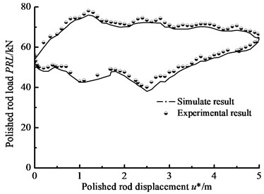
A wireless indicator is installed between polished rod and SRS, in Fig. 5. With the indicator, the surface dynamometer card is obtained in Fig. 6. Based on the simulation model of surface driving units [2] and the improved simulation model in this paper, the dynamic response of beam pump system is obtained with above basic parameters. In the detail, the simulation model of two degree of freedom torsional vibration for surface driving system is built, and the equivalent rotational inertia of two discs are derived with the masses and rotational inertia of every moving part for surface driving system [2]. Combining the simulation models of surface and down-hole system, the numerical model of beam pump system is solved with Runge-Kutta method. And the surface dynamometer card is obtained in Fig. 6.

According to the Fig. 6, the maximum and minimum polished rod loads of the measured curve are 78.14 kN, 38.71 kN, and the maximum and minimum polished rod loads of simulation curve are 76.01 kN, 37.13 kN. The relative errors of measured and simulate curves are 2.73 %, 4.08 %. In the up and down stroke, the maximum and minimum relative errors between the measured curve of the polished rod load and the simulation curve are 4.86 %, 0.71 %. The simulation curves of the dynamometer card based on the new model are found to be in good agreement with the experimental curves. Therefore, the new model in this paper is accurate enough to be used for engineering practice.

Fig. 5The wireless indicator

Fig. 6Comparison of the numerical solution with experimental load–displacement curve

4.2. Affecting factors of plunger load

4.2.1. Hydraulic loss

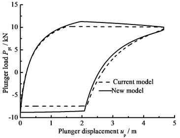
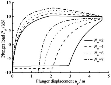
When the clearance leakage between pump plunger and pump barrel $Q_t=$0, the influence of the hydraulic loss on the plunger load is only considered and the comparison curves of pump plunger load with no hydraulic loss or hydraulic loss are given in Fig. 7(a). In Fig. 7(b), the comparison curves of pump plunger load with current model or new model are given. When other parameters do not change, considering the influence of stroke number and power law exponent on hydraulic loss, the curves of pump plunger load with different stroke number are given in Fig. 7(c), and the curves of pump plunger load with different power law exponents are given in Fig. 7(d).

Fig. 7The influence of hydraulic loss on plunger load

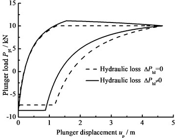
a) Influence of hydraulic loss

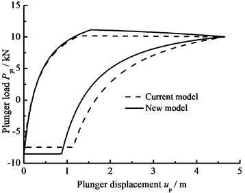
b) Comparison of current and new model

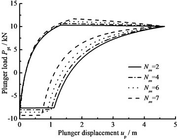
c) Stroke number

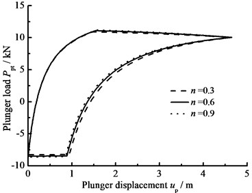
d) Power law exponent

As you can see in the above figures, when the hydraulic loss is taken into consideration, the maximum load of pump plunger increases and the minimum load of pump plunger decreases. With increasing stroke number and power law exponent, the maximum load of pump plunger is increasing and the minimum load of pump plunger is decreasing. In addition, the area of pump diagram is decreasing with stroke number and power law exponent increasing.

Fig. 8The influence of clearance leakage on plunger load

a) Influence of clearance leakage

b) Comparison of current and new model

c) Stroke number

d) Power law exponent

e) Gap between plunger and pump barrel

f) Consistency coefficient

4.2.2. Clearance leakage

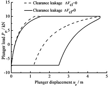
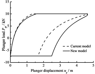
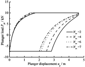
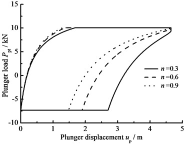
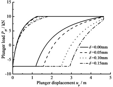
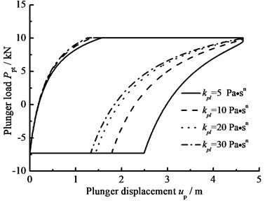
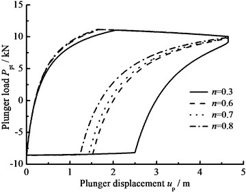
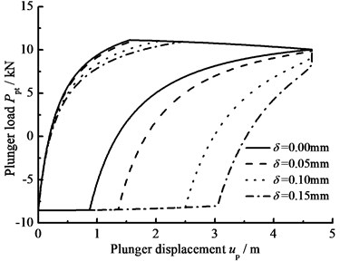
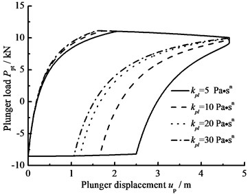
When the hydraulic loss of pump valve $\mathrm{\Delta }P=$0, the influence of the clearance loss between pump plunger and pump barrel is only considered and the comparison curves of pump plunger load with no clearance leakage or clearance leakage are given in Fig. 8(a). In Fig. 8(b), the comparison curves of pump plunger load with current model or new model are given. When other parameters do not change, considering the influence of some parameters on clearance leakage, the curves of plunger load with different parameters are given, such as stroke number, power law exponent, consistency coefficient and gap between plunger and pump barrel, in Fig. 8(c), (d), (e), (f).

In Fig. 8, when the clearance leakage between pump plunger and pump barrel is taken into consideration, the falling rate of liquid pressure is decreasing in the up stroke. Therefore, the standing valve opens with short delay. On the other hand, the increasing rate of liquid pressure is increasing in the down stroke, so the traveling valve opens in advance. With stroke number, power law exponent and consistency coefficient decreasing, the lagged time of standing valve opening is increasing and the lead time of traveling valve opening is decreasing. In addition, with the gap between pump plunger and pump barrel increasing, the lagged time of standing valve opening is increasing and the lead time of traveling valve opening is decreasing.

Fig. 9The influence of hydraulic loss and clearance leakage on plunger load

a) Influence of hydraulic loss and clearance leakage

b) Comparison of current and new model

c) Stroke number

d) Power law exponent

e) Gap between plunger and pump barrel

f) Consistency coefficient

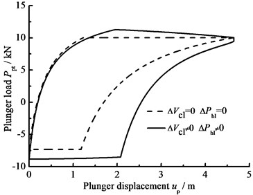
4.2.3. Hydraulic loss and clearance leakage

The influence of hydraulic loss of pump valve on plunger load as well as the influence of clearance leakage between pump plunger and pump barrel is considered, the comparison curves of plunger load with no hydraulic loss or clearance leakage are given in Fig. 9(a). In Fig. 9(b), the comparison curves of pump plunger load with current model or new model are given. When other parameters do not change, with the influence of some parameters on plunger load, the curves of plunger load with different parameters are given, such as stroke number, power law exponent, consistency coefficient and gap between plunger and pump barrel, in Fig. 9(c), (d), (e), (f). As see in Fig. 9, considering the influence of hydraulic loss and clearance leakage on plunger load, the standing valve opens with short delay and the maximum load of pump plunger increases in the up stroke. In the down stroke, the traveling valve opens in advance and the minimum load of pump plunger decreases. With the stroke number decreasing, the lagged time of standing valve opening is increasing and the maximum load is decreasing in the up stroke, the lead time of traveling valve opening is decreasing and the minimum load is increasing in the down stroke. In addition, with the power law exponent and consistency coefficient decreasing, the lagged time of standing valve opening is increasing in the up stroke, the lead time of traveling valve opening is decreasing in the down stroke. When the gap between pump plunger and pump barrel is decreasing, the lagged time of standing valve opening is decreasing in the up stroke, the lead time of traveling valve opening is increasing in the down stroke.

4.3. Impact analysis of SRS absorber

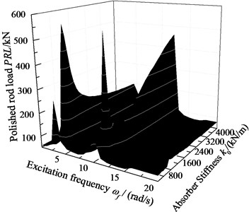
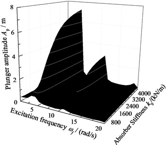
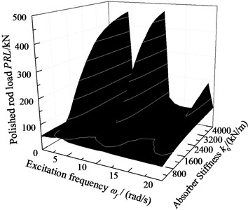
When $c_0=$6.0×10⁵ N·s/m, $k_0=$2.0×10⁶ N/m, the displacement of pump plunger and load of polished rod are simulated. In addition, the plunger displacement and polished rod load are also obtained with no SRS absorber. The relative curves of displacement and load are given in Fig. 10. When $c_0=$0 and other parameters do not change, the excitation frequency and stiffness of SRS absorber are changed simultaneously, the three-dimensional curves of plunger displacement and polished rod load are obtained in Fig. 11. When $c_0=$6.0×10⁵ N·s/m and other parameters do not change, the excitation frequency and stiffness of SRS absorber are changed simultaneously, the three-dimensional curves of plunger displacement and polished rod load are obtained in Fig. 12.

Fig. 10The amplitude-frequency curve

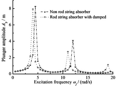
a) Pump plunger displacement

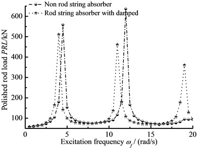
b) Polished rod load

As you can see in figures, when the SRS absorber is ignored, there are two resonance points in the frequency range of 0 to 20 rad/s. But there are there resonance points in same frequency range with SRS absorber, which is a major characteristic of nonlinear vibration. In addition, the polished rod load decreases in non-resonant region when the SRS absorber is considered. The influences of excitation frequency and absorber stiffness on the plunger displacement and polished rod load are intuitively expressed in three-dimensional curves. The above conclusions are very important to the design of the SRS absorber in practical applications.

Fig. 11The amplitude-frequency with no damped absorber

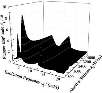
a) Pump plunger displacement

b) Polished rod load

Fig. 12The amplitude-frequency with damped absorber

a) Pump plunger displacement

b) Polished rod load

5. Conclusions

The following conclusions can be summarized from the theoretical formulation and the numerical studies in this paper:

1) Considering the influence of nonlinear characteristic of SRS friction and plunger load on the SRS’s longitudinal vibration, an improved simulation model of longitudinal vibration for mix absorber with SRS is built. In the detail, selecting NNPLF as the research object, some new models are established, such as the nonlinear friction between pump plunger and NNPLF, the hydraulic loss of pump and the clearance leakage between pump plunger and pump barrel. The dynamic responses are obtained with zero initial conditions based on fourth order Ronge-Kutta method.

2) In order to verify the feasibility of the proposed dynamics simulation model, the wireless indicator is used. It shows that the simulated and experimental results of polished rod load have a good match.

3) Considering the influence of hydraulic loss and clearance leakage on the instantaneous liquid pressure of pump, the influences of some parameters on the pump plunger load are analyzed, such as stroke number, power law exponent, consistency coefficient and the gap between pump plunger and pump barrel. The results show that when the stroke number is increasing, the maximum load of pump plunger is increasing and minimum load of pump plunger is decreasing. With the stroke number, the power law exponent and consistency coefficient decreasing, the lagged time of standing valve opening is increasing in the up stroke, the lead time of traveling valve opening is decreasing in the down stroke. In addition, when the influence of SRS absorber on SRS’s longitudinal vibration is taken into consideration, there is an obvious characteristic of nonlinear longitudinal vibration. The above conclusions are very important to system fault diagnosis and the design of the SRS absorber in practical applications.