Research on speed’s influence on hydrostatic bearing’s stiffness

Changting, Chen; Jinfu, Yang; Dongjiang, Han; Changliang, Tang

Vibroengineering Procedia

Browse Procedia

Published: 03 November 2014

Check for updates

Research on speed’s influence on hydrostatic bearing’s stiffness

Chen Changting¹

Yang Jinfu²

Han Dongjiang³

Tang Changliang⁴

^{1, 2, 3, 4}Institute of Engineering Thermophysics, Chinese Academy of Sciences, Beijing, China

Corresponding Author:

Chen Changting

Cite the article Download PDF

Downloads 1335

Abstract

Reynolds equation considering speed is solved using finite element method. Orifice hydrostatic gas bearing’s pressure distribution, load capacity and stiffness are obtained. Speed’s influenced on stiffness is studied. Experiment is conducted on turbine expander. Rotor operates under unbalance mass’s excitation. By analysis whipping frequency’s relation with the natural frequency of rotor-bearing system, stiffness can be calculated. The experiment result shows that bearing’s stiffness changes with rotor’s speed. When rotor’s speed is between 10000-50000 r/min, stiffness increased by 9.6 %. Because gas whirl only happens when rotor’s speed is above the first critical speed, the method has limited speed range.

1. Introduction

Aerostatic bearings are commonly used in high speed rotating equipments due to its advantages such as low friction, low heat and environmentally friendly [1, 2]. Gas stiffness is one of bearing’s property. Conventionally, measurement of stiffness is in the stationary state. Under uploading condition, static stiffness can be determined through measuring bearing’s capacity and film thickness [3-5]. Although the aerostatic bearing mainly depends on the supply pressure, the effect of dynamic pressure in high speed cannot be ignored [6].

The paper puts up a new method to measure bearing’s stiffness and researches speed’s influence on stiffness. The experiment is conducted on turbine expander supported by gas hydrostatic bearing. When rotor accelerates, the rotor will have unbalance response and gas film whipping happens under certain condition. By analysis whipping frequency’s relation with the natural frequency of rotor-bearing system, stiffness can be calculated. At the same time, finite element method is used to slove the Reynolds equation to obtain bearing’s stiffness. Comparison between theoretical value and experimental value is done.

2. Calculation of stiffness

2.1. Reynolds equation

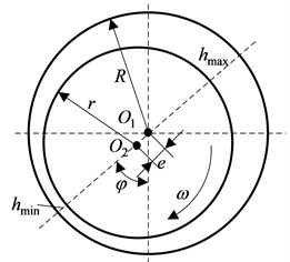
Considering hydrostatic bearing’s dynamic effect shown in Fig. 1, rotor runs in the speed of $ω$ . Where $O_{1}$ is bearing’s center, $O_{2}$ is rotor’s center, $e$ is eccentricity, $h_{m} = R - r$ is film thickness, $φ$ is angle of displacement.

Suppose gas is in isothermal condition, gas lubrication equation considering speed’s effect is:

1

\frac{\partial}{\partial x} (h^{3} \frac{\partial p^{2}}{\partial x}) + \frac{\partial}{\partial z} (h^{3} \frac{\partial p^{2}}{\partial z}) + 12 η ρ \frac{ρ_{a}}{p_{a}} δ_{i} = 6 η ω \frac{\partial (p h)}{\partial x},

where $η$ is gas’s viscosity, $ρ$ is gas’s density, $ρ_{a}$ atmospheric density, $p_{a}$ is atmospheric pressure. Establish dimensionless form of Eq. (1):

2

\frac{\partial}{\partial \bar{x}} ({\bar{h}}^{3} \frac{\partial {\bar{p}}^{2}}{\partial \bar{x}}) + \frac{\partial}{\partial \bar{z}} ({\bar{h}}^{3} \frac{\partial {\bar{p}}^{2}}{\partial \bar{z}}) + \bar{Q} δ_{i} = Λ \frac{\partial (\bar{p} \bar{h})}{\partial \bar{x}},

where $\bar{p} = p / p_{0}$ is dimensionless pressure, $\bar{h} = h / h_{m}$ is dimensionless film thickness, $\bar{x} = x / L$ is dimensionless displacement of $x$ , $\bar{z} = z / L$ is dimensionless displacement of $z$ , $Λ = 12 μ ω l / h_{m}^{2} p_{0}$ is bearing number, $\bar{Q} = 24 μ l^{2} p_{a} / h_{m}^{3} p_{0}^{2} ρ_{a} ρ \tilde{v}$ is gas mass flow factor through orifice, ${\bar{δ}}_{i}$ is Kronecker delta function which equals to 1 in orifice region and 0 in other region.

Fig. 1Bearing’s dynamic pressure film

The expression of mass flow is given by:

3

\dot{m} = A p_{0} ϕ \sqrt{\frac{2 ρ_{0}}{p_{0}}} ψ,

where:

ψ = \{\begin{array}{l} {[\frac{k}{2} {(\frac{2}{k + 1})}^{\frac{k + 1}{k - 1}}]}^{\frac{1}{2}} ， \frac{p}{p_{0}} \leq β_{k}, \\ {[\frac{k}{k - 1} [{(\frac{p}{p_{0}})}^{2 / k} - {(\frac{p}{p_{0}})}^{k + 1 / k}]]}^{\frac{1}{2}} ， \frac{p}{p_{0}} > β_{k}, \end{array}

and $ϕ$ is mass flow loss factor which equals to 0.8 to considerate errors between real and theoretical value.

2.2. Solve of Reynolds equation

2.2.1. Discretion of Reynolds equation

Discrete Reynolds equation using Galerkin method [3]. Film field is divided into a grid size of $m$ elements and $n$ nodes. The integral in whole area is equal to the sum of each element. The equation can be written as:

4

\sum_{e = 1}^{m} \int_{Δ e} {\bar{h}}^{3} [\frac{\partial f}{\partial \bar{x}} \frac{\partial δ f}{\partial \bar{x}} + \frac{\partial f}{\partial \bar{z}} \frac{\partial δ f}{\partial \bar{z}}] - \bar{Q} δ_{i} δ f - Λ f^{\frac{1}{2}} \bar{h} \bar{ω} \frac{\partial δ f}{\partial \bar{x}} d \bar{x} d \bar{z} = 0,

$f$ is replaced by interpolation function. Choose triangle element as interpolation function. $\bar{Q} δ_{i} δ f$ has value only in orifice area and the outlet pressure of orifice is $p_{d r}$ . Eq. (4) becomes:

5

\sum_{e = 1}^{m} \int_{Δ e} \bar{Q} δ_{i} δ f d \bar{x} d \bar{z} = \sum_{A \in Ω} \frac{24 η p_{a} f_{d r}}{h_{m}^{3} p_{0}^{2} ρ_{a}} δ_{i} \int_{A} ρ \tilde{ν} d \bar{x} d \bar{z},

$\int_{A} ρ \tilde{ν} d \bar{x} d \bar{z}$ is mass flow ${\dot{m}}_{A}$ which can be written as:

6

K_{1} \sum_{A \in Ω} f_{d r} {\dot{m}}_{A} δ_{i},

where $K_{1} = 24 η p_{a} / h_{m}^{3} p_{0}^{2} ρ_{a}$ .

One can rearrange Eq. (4) using interpolation function as follows:

7

\begin{array}{l} \sum_{e = 1}^{m} δ f^{e T} \int_{Δ e} [{(N^{e T} h^{e})}^{3} (\frac{\partial N^{e}}{\partial \bar{x}} \frac{\partial N^{e T}}{\partial \bar{x}} + \frac{\partial N^{e}}{\partial \bar{z}} \frac{\partial N^{e T}}{\partial \bar{z}}) f^{e} - \bar{Q} N^{e} δ_{i} \end{array}

- λ \frac{\partial N^{e}}{\partial \bar{x}} \bar{u} h^{e T} N^{e} N^{e T} {(f^{\frac{1}{2}})}^{e}] d \bar{x} d \bar{z} = 0 .

In order to getting limiting value, let $δ f = 0$ in Eq. (7). Because $\partial N_{i} / \partial x$ , $\partial N_{i} / \partial z$ , $\partial N^{e T} / \partial x$ , $\partial N^{e T} / \partial z$ is rectifiable, we can write function as follows:

8

K F = T .

The right-hand member of Eq. (8) contains unknown parameter, so it is a nonlinear equations.

2.2.2. Solution of nonlinear equations

SOR iteration method is adopted to solve the Eq. (8). Generally, the direction of bearing’s load capacity is vertical. That requires the force of vertical is much bigger than force in horizontal direction. For initial condition, angle of displacement is supposed to be $φ_{0}$ and is updated until $|W_{x} / W_{y}| \leq δ$ is satisfied. Iterating equation is:

9

φ_{n e w} = φ_{o l d} - t a n^{- 1} |W_{x} / W_{y}| .

2.2.3. Mesh generation

Expand film in the direction of circumferential as shown in Fig. 2. Element’s length is defined according to calculation precision. In this paper, circumferential direction is divided into 17 and $d x = π / 8$ ; axial direction is divided into 7 and $d z = 1/6$ .

The total number of film field is 119.Calculation field is numbered from 1 to 102. Number 103 to 109 are satisfied with atmosphere boundary condition which is $p = p_{a}$ . Orifice holes locate in 4, 16, 28, 40, 52, 64, 76, 88.

2.2.4. Bearing’s structure parameters

Calculate orifice externally pressurized gas bearing’s pressure distribution, load capacity and stiffness. Bearing’s structure parameters and lubrication gas’s features is listed in Table 1.

Fig. 2Calculation field’s element

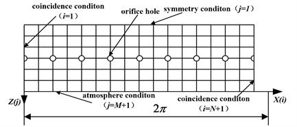
Table 1Bearing’s parameters

Parameter	Symbol/unit	Value
Length of bearing	$L$ / mm	37.5
Diameter of bearing	$D$ / mm	25
Number of orifices	–	16
Diameter of orifices	$d$ / mm	0.8
Throttle coefficient	–	0.8
Distance between orifices	$L_{1}$ / mm	17.5
Supply pressure	$p_{0}$ / MPa	0.6

2.2.5. Calculation result and analysis

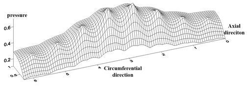
Fig. 3 shows dimensionless film thickness in the direction of circumferential. Fig. 4 shows dimensionless pressure distribution. From the results we can see that every orifice’s pressure is the same without eccentricity. When the eccentricity increases, pressure difference becomes bigger. Pressure increase with the decease of film thickness.

Stiffness is calculated under different speeds. When the speed are 10000 r/min-50000 r/min, stiffness is 1.215×10⁶N/m to 1.4×10⁶N/m which increases by 15.2 %.

3. Experiment scheme and calculation method

3.1. Experiment scheme

When sliding bearing supported rotor works higher than the first critical speed, the rotor is prone to occur whipping which the frequency is the same with rotor-bearing system’s natural frequency. If the rotor-bearing system’s natural frequency does not change, the frequency of whipping will not change which is often called oscillation frequency lock [7-9].

Rotor supported by bearing’s natural frequency is $ω = \sqrt{K / M}$ . $K$ is rotor-bearing system’s stiffness and $M$ is mass. Two bearing are connection in parallel, then connection in series with rotor. $K$ is calculated as follows:

10

K = \frac{2 k_{f} k_{r}}{2 k_{f} + k_{r}},

where $k_{f}$ is film’s stiffness and $k_{r}$ is rotor’s stiffness. Natural frequency of rotor-bearing system is $f$ is experimental resonant frequency. We can get the value of $K$ from the expression:

11

K = M ω^{2} = M (2 π f)^{2} .

Fig. 3Dimensionless film thickness distribution

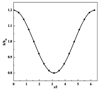
Fig. 4Dimensionless pressure distribution of gas film

3.2. Introduction of experiment lab

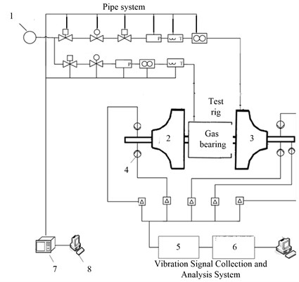
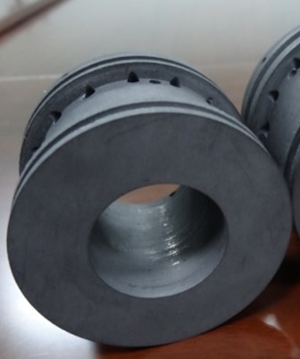
Experiment is done on turbo expander. Rotor is driving by gas turbine. The speed is controlled by changing the gas flow. A gas turbine expander and its system is shown in Fig. 5. Rotor is supported by gas bearing. Gas bearing is made of graphite alloy. Rotor is powered by high pressure gas driving the turbine which ranges from 0.1-1.3 MPa. Eddy current displacement sensors are placed in both compressor and turbine side in horizontal and vertical direction to collect the rotor vibration signal. Another sensor is arranged in the shaft to collect speed signal.

Fig. 5Controlling testing and analyzing system for turbo-expander and testing bearing

a)

b)

3.3. Calculation of rotor’s stiffness

Test rotor is stepped form which is shown in Fig. 6. In order to get moment of inertia of cross-section, rotor is discreted and is calculated using the equivalent moment of inertia.

Rotor’s stiffness is $9.347×1 0^{6} N/m$ .

3.4. Calculation of bearing’s stiffness

Fig. 7 is time, frequency and amplitude three dimensional spectrum of speeding up experiment. Rotor’s highest speed is 60180 r/min. Low frequency vibration occurs when power frequency is 791 Hz (47460 r/min) and disappears until 1003 Hz (60180 r/min). As shown in Fig. 7, line AB refers to low frequency vibration ranges from 230 Hz-250 Hz.

Fig. 6Rotor’s structure

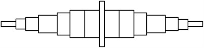
Fig. 7Time-frequency-amplitude three-dimensional spectrum of speeding up experiment

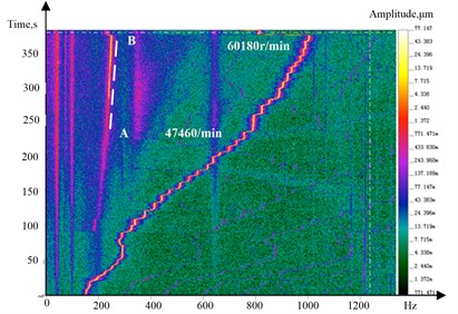
Fig. 8 is rotor’s orbit in vibration area. We can infer that oscillation vibration happens. With the increase of power frequency, oscillation frequency increase.

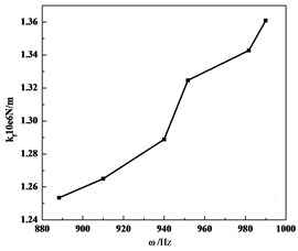
Fig. 9 is bearing’s stiffness when rotor’s speed is 880 Hz to 990 Hz, we can see that film’s stiffness increased by 9.6 %.

Fig. 8Rotor’s orbit in vibration area

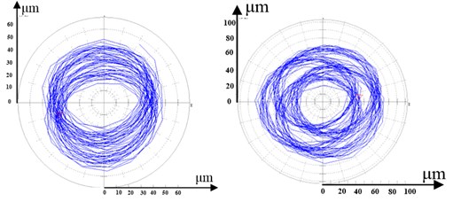
Fig. 9Bearing’s stiffness

4. Conclusions

In this work, a new experimental method is put up to test bearing’s dynamic stiffness. Sometimes when rotor accelerates, whipping happens. Dynamic stiffness is extracted from whipping frequency. From the study we can get the following conclusions.

1. The stiffness is calculated through solving Reynolds equation considering speed. The result shows that when rotor’s speed is between 10000-50000 r/min, stiffness increased by 9.6 %.

2. The experimental result also shows that film’s stiffness increases with rotor’s speed and has influenced on rotor-bearing’s critical speed.

3. The method can measure bearing’s dynamic stiffness. Because gas whirl only happens when rotor’s speed is above the first critical speed, the method has limited speed range.

References

Chen Rugang, Hou Yu, Yuan Xiuling Application of gas bearing on high speed turbo-machinery. Journal of Fluid Mechanics, Vol. 35, Issue 4, 2007, p. 28-32.

Search CrossRef
Shi Hejinyi The design, manufacture and application of gas bearing. China Astronautic Publishing House, Beijing, 1988, (in Chinese).

Search CrossRef
Liu Dun, Liu Yuhua, Chen Shijie Aerostatic bearing. Harbin Institute of Technology Press, Haerbin, 1990, (in Chinese).

Search CrossRef
Wu Qi Research on static and dynamic characteristic of aerostatic bearing used in high-precision spindle. Harbin Institute of Technology, Haerbin, 1995, (in Chinese).

Search CrossRef
Zhao Huiying, Tian Shijie, Jiang Zhuangde Rigidity analysis on high-presion aerostatic bearing system. Manufacturing Technology and Machine Tool, Vol. 11, 2003, p. 21-23, (in Chinese).

Search CrossRef
Lo C. Y., Wang C. C., Lee Y. H. Performance analysis of high-speed spindle aerostatic bearings. Tribology International, Vol. 38, Issue 1, 2005, p. 5-14.

Search CrossRef
Yang Jinfu, Yang Shengbo, Chen Ce Research on sliding bearings and rotor system stability. Journal of aerospace power, Vol. 23, Issue 8, 2008, p. 1420-1426, (in Chinese).

Search CrossRef
Guo Jun, Liu Baoyu, Yang Jinfu An experiment research on the control of sub-synchronous coupling whirl characteristics of gas lubrication bearings rotor system. Lubrication Engineering, Vol. 35, Issue 3, 2010, p. 86-89, (in Chinese).

Search CrossRef
Han Dongjiang, Yang Jinfu, Zhao Chen An experiment study on vibration characteristics for gas bearing-rotor system. Journal of Vibration Engineering, Vol. 25, Issue 6, 2012, p. 1199-1203, (in Chinese).

Search CrossRef

About this article

Received

Accepted

05 August 2014

Published

03 November 2014

Keywords

hydrostatic bearing

FEM

bearing’s stiffness

oscillation vibration

This is an open access article distributed under the Creative Commons Attribution License, which permits unrestricted use, distribution, and reproduction in any medium, provided the original work is properly cited.