Abstract
Satellite geodetic measurements used in the diagnosis of railway tracks require professional receivers and a very high frequency rate of data processing. It stems from a significant speed (10 km/h) kinematic measurements carried out during the passage of a measuring platform. The survey results (positions) of deformed railroad track have waveforms nature requiring additional processing methods and approximations. Due to the announcement in 2011 of the operating status for the Russian Global Navigation System (Glonass) and launching a commercial geodetic satellite network SmartNet in northern Poland (2012) created for the first time a possibility of carrying out measurements using two satellite systems (GPS/GLONASS) which significantly increase the accuracy of measurements on a rail. A paper presents a possibility of using two-system satellite receivers to measure the deformation of the tram track on the example of the measurement line in Gdansk (October 2013). The studies used rarely encountered in geodesy a very high position frequency rate (20 Hz), which entails the use of wave processing methods.
1. Introduction – development of satellite surveying methods
The Navstar Global Positioning System, hereafter referred to as GPS, is a space-based radionavigation system owned by the United States Government (USG) and operated by the United States Air Force (USAF). GPS has provided positioning, navigation, and timing services to military and civilian users on a continuous worldwide basis since first launch in 1978. An unlimited number of users with a civil or military GPS receiver can determine accurate time and location, in any weather, day or night, anywhere in the world. In 1983 the U.S.A. President Ronald Reagan announced civil users would be granted access to Standard Positioning Service (SPS) which broadcasts code signals (C/A – Coarse/Acquisition) at L1 frequency that can be used to determine time the position of a receiver, once it became operational. Due to initial military designation of GPS, SPS accuracy for unauthorized, civil users was deliberately degraded with the technique called Selective Availability (SA). Full Operational Capability (FOC) was declared by Air Force Space Command (AFSPC) in April 1995. On May 1, 2000, President Clinton announced the discontinuance of SA effective midnight 1 May 2000. The effects of SA went to zero at 0400 UTC on 2 May 2000 [1]. Until 2011, the GPS system based on a constellation of 30 satellites was the only global positioning system used in surveying. Today GPS is the main source of position solutions to a wide range of geodesy and navigational applications. Current positioning accuracy for navigation can be estimated as: 2.961 m (0.95) horizontally and 6.902 m vertically ( 0.95) [2].
Besides the navigation applications, GPS has found its wide use in geodesy, for example in applying navigation surveying system software using the technique of relative measurements performed by two receivers. One of the them (reference station) was located on a point with known coordinates and the second one (called rover station) on a point whose position had to be determined. This solution has been used successfully in the 1990s. It ensures the feasibility of measuring a distance of 30 km from the reference station. The main disadvantage of this solution was a decrease in the accuracy of assignments position with the distance between the devices which was 2 cm 1 ppm. This means that at a distance of 20 km from a reference station accuracy was about 6 cm. For this reason, she did not meet the requirements for geodetic measurement systems used in the railway industry. A significant change occurred in the early 1900s, when state institutions responsible for surveying began the process of creating a national GPS network solutions. Principal advantage of this network solution is the possibility of reducing the measurement error resulting from the distance between the reference station and the receiver by using a measurement technique of Virtual Reference Station. The GPS network decides from the rover’s location, which reference stations data, best suited, will be used in position correction. For users they only need to connect to the network by automatically sending their navigated position via the NMEA GGA string, which is pre-configured in the rover sensor. The network will then return the corrections to the user with the optimum stations for their location.
Today, there are two official accepted standard protocols for transmitting DGNSS data in satellite active geodetic networks over the internet: Networked Transport of RTCM via the Internet Protocol (NTRIP) and Real-Time IGS (RTIGS). They are used for real time differential transmissions over the active geodetic networks. NTRIP was developed using the principles of an internet radio technology to support dissemination of DGNSS data over the internet in real-time. NTRIP is a generic, stateless protocol based on the Hypertext Transfer Protocol HTTP/1.1. A few years ago the RTCM Committee accepted NTRIP version 1.0 as a standard for packet-based communications [3]. NTRIP version 1.0 utilizes Transmission Control Protocol and Internet Protocol (TCP/IP) to obtain a reliable delivery of byte streams. NTRIP version 2.0 is undergoing evaluation for full HTTP compatibility and for the optional use of the User Datagram Protocol and IP (UDP/IP) in addition to TCP/IP. NTRIP can be used not only for ‘carrying’ RTCM format data, but also other proprietary GNSS data formats. The main problem related to active geodetic network positioning is to solve spatial distribution of the dominanted errors as ionospheric delay, tropospheric delay and orbit error. The errors are classified as dispersive (ionosphere) and non-dispersive (troposphere and orbit).
2. GNSS active geodetic network railway application
In 2009, Gdansk University of Technology and the Naval Academy created a team dedicated to research inventory of railways and designing their geometries. Its members included academics Gdansk University of Technology and Naval Academy in Gdynia, with the cooperation of the Polish Railway Lines – Railways Department in Gdynia. The first study was carried out in 2009 on the 50-km-long railway line Koscierzyna-Kartuzy. The next two measurements carried out in 2010 in the center of Gdansk and the Gdansk-Osowa- Koscierzyna. First measurements of the railway lines were carried out in Gdansk in February 2010. From the beginning of the research until now, the method has been successfully improving [4, 5].
In 2009-2010, to determine the coordinates of the route, the Polish Railways used different configurations of phase GNSS receivers, including their number and arrangement of the measuring platform. The first measurement (2009) used the 4 GPS devices system placed in the rectangle directly above the rear wheels. These studies [6] have shown that a crucial element of the accuracy of the position coordinates were Iris Field (availability of items with errors of less than 5 cm was approximately 50 %). In subsequent measurements, searching for the optimal location of instruments deployed three receivers diametrically measuring carriage. Tests have shown similar availability and accuracy of GPS space segment for all units of measurement, but still achieved the level of availability of appointments for the measurement error of less than 5 cm reached unsatisfactory values (60-70 %). After a detailed analysis of the conditions of the measurements carried out in 2009-2010, it was decided to thoroughly verify the methodology, whereby:
– The surveyors abandoned the implementation of real-time measurements using the ASG-EUPOS, due to the existing gap in the work of the network associated with the transmission of GPS pseudorange corrections. In the afternoon, a large number of users caused a disconnection of service users packet data (GPRS);
– The instability of the network ASG-EUPOS led the authors to the decision to resign from the measurements in real time. It was decided to implement them in post-processing, making development results gave greater freedom to use signals of different reference stations;
– To improve the accuracy of the positions directly related to the number of available GPS satellites, it was decided to implement measurement using dual-mode GNSS receivers, thus utilizing the signals of two satellite systems: GPS and Glonass.
Table 1GNSS measuring sets configurations used for the diagnosis of railway tracks. Methods evolution
2009 February | Railway routes: Koscierzyna-Kartuzy – 50 km 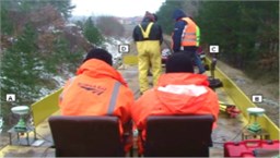 | GNSS Solution: GPS only, ASG-EUPOS Network, VRS, FKP, MAC Processing: Real Time, Service NAVGEO, Distance auto-recording 30 cm, Leica Office software Receivers: 4 phase GPS (Leica ATX 1230GG) 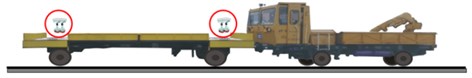 |
2010 April | Railway routes: Gdansk-Osowa-Koscierzyna – 20 km  | GNSS Solution: GPS only, ASG-EUPOS Network, VRS, FKP, MAC Processing: Real Time, Service NAVGEO, Distance auto-recording 30 cm, Leica Office software Receivers: 3 phase GPS (Leica ATX 1230GG) 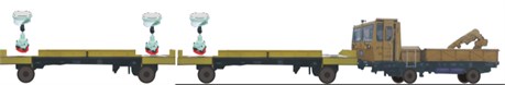 |
2010 November | Railway routes: Gdansk-Osowa-Koscierzyna – 60 km 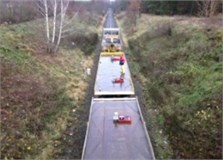 | GNSS Solution: GPS only, ASG-EUPOS Network, VRS Processing: Real Time, Service NAVGEO, Distance auto-recording 30 cm, Leica Office software Receivers: 3 phase GPS (2xLeica ATX 1230GG, 1x Leica GS 15)  |
2012 February | Tramp routes in Gdansk – 50 km of tramp lines  | GNSS Solution: GPS/Glonass, FKP from station located in Gdansk Technical University Processing: Post-processing, Auto-recording every 30 cm, data analyses in Leica Office software Receivers: 2 phase GPS/Glonass (Leica GS-12, Leica GS 15) |
 |
Russian GLONASS, is a space-based Global Positioning System (GPS) operated by the Russian Aerospace Defence Forces. It is the Russian version of America’s military GPS and is currently the only alternative navigational system in operation capable of global coverage. Russian GLObal NAvigation Satellite System project started in 1976 based on Decree of the Soviet Union Communist Party Central Committee and Council of Ministers of the USSR. In March 1995, the system achieved full operational capability, however, the disintegration of the Soviet Union (1988-1991) caused a loss of the ability to provide the required number of satellites in the constellation. In 1998, by a decree of the President of Russia the plan re-expansion of the system was accepted. The GLONASS program obtained significant support in May 2007 when the Decree of the President of the Russian Federation was issued. The President made commitments to sustain the GLONASS system and provide its open service free of charge and available for all civilian users worldwide without any restrictions. At the same time the Government of the Russian Federation accepted the system development program for 2020. Since December 2011, the GLONASS system has been fully operational, providing worldwide service with 99.8 percent global availability and acceptable accuracy for users. Currently (February 2014) satellite constellation consists of 28 pieces which significantly supplements the possibility to implement integrated GPS/Glonass measurements [7].
3. Campaign and results
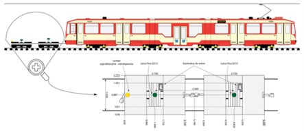
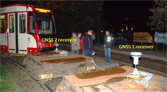
Surveying tram routes in Gdansk was completed on September 20-21, 2013. For the first time two geodetic satellite systems: GPS and Glonass and private active satellite geodetic network were used for this purpose. Thanks to the announcement in 2011 of the operating status for the Russian Global Navigation System (Glonass) and opening in the northern Poland a commercial geodetic satellite network SmartNet (2012), for the first time it was possible to carry out measurements, using two satellite systems (GPS/GLONASS) which significantly increased the accuracy of measurements on a rail. Leica SmartNet is the Polish first commercial network which provides for a corrections service for any professional GPS/Glonass receivers. The study was conducted at night (11:30 pm-05:30 am), in order to avoid any conflict with the commercial activities of public transport. Two GPS receivers Leica GS-15 and GS-12 with standard accuracies 10 mm (rms) were used to carry out measurements. Measuring exact positioning of antennas receivers in the centre of the track tram was made with the use of the geodetic total station Leica TCRA 1103. By using the total station was defined baseline – defined by the axis tram track. Estimated antenna positioning accuracy was less than 1 mm (Fig. 1).
Fig. 1Configuration of GPS/Glonass receivers on the platform
Data files were containing position time series in the format referenced to World Geodetic System WGS-84 datum (6378137.00 m, 6356752.314 m). The World Geodetic System 1984 (WGS84) datum is the nominal datum used by GPS [8]. It is based on the WGS84 ellipsoid which only exhibits a small difference in the flattening parameter compared to the GRS80 and therefore both ellipsoids can be assumed identical for most practical purposes. To obtain the coordinates in meters measured ellipsoidal coordinates were transformed to Gauss-Kruger (, ) conformal coordinates (in meters), based on relations:
where: , – measured ellipsoidal GPS/Glonass coordinates; – radius of curvature in the prime vertical; – distance from the equator to defined coordinate ; – difference in longitude between and prime meridian; 0.999923 – scale factor.
Others parameters could be calculated as:
where: – eccentricity of WGS-84 ellipsoid; – orientation angle of WGS-84 ellipsoid.
Fig. 2Cross Track Error as a function of longitude for test-size 70-meter section of tramp track
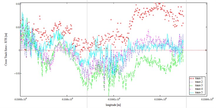
The collected data were transformed to local coordinate system, in which the horizontal axis states direction consistent with the axis of track on a straight section. Therefore, the values different from zero on the vertical axis state the deviation of the GPS/Glonass signal from the direction of the measured route. If the measurement was conducted at the perfectly straight track (with a specified accuracy of horizontal inequality), the recorded samples would represent the value of the measurement error, which would determine the accuracy of adopted methodology. However in practice, the situation is that track’s axis tends to be deformed as a result of operating and technological processes, aimed at the track maintenance. It is therefore expected that the measured signal transformed to such system (after transformation) will represent the deformation of the track in relation to the design assumptions. In navigational terms, the position of navigated object at a distance from the established course (as assumed direction) in the lateral direction is called as XTE (Cross Track Error), and it states one of the measure of the position errors of a moving object. As we can see, on the railway a very similar phenomenon occurs. Therefore we can also describe the horizontal irregularity of the track with the use of the function of XTE for this purpose. Then the results (XTE) of the transformation coordinates for test-size 70-meter section of track were analyzed. This testing part of the track was measured five times. The XTE values (for 5 passes) related to the approximation tramp line is presented below.
The statistical analysis shows that XTE can be modeled by formula:
where (XTERough) is the remainder (irregular) component and is the trend-cycle component at place (period ). Fig. 3 shows various statistics for the variable samples, [9].
Fig. 3The Box and Whisker plot of the 5 columns of data
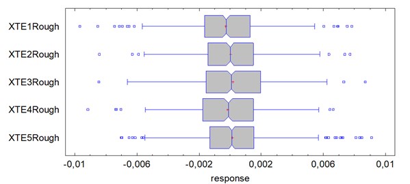
The Box-and-Whisker Plot (Fig. 3), summarizes a data sample through 5 statistics minimum, lower quartile, median, upper quartile, maximum [10]. A box is drawn extending from the lower quartile of the sample to the upper quartile. This is the interval covered by the middle 50 % of the data values when sorted from smallest to largest. A vertical line is drawn at the median (the middle value). A notch is added to the plot showing an approximate 95 % confidence interval for the median. A plus sign is placed at the location of the sample mean. Whiskers are drawn from the edges of the box to the largest and smallest data values, unless there are values unusually calls outside points. Outside points, which are points more than 1.5 times the interquartile range (box width) above or below the box, are indicated by point symbols. The whiskers are drawn to the largest and smallest data values which are not outside points.
Table 2The fitted distribution parameters and the results of goodness tests
Data variable | Fitted distributions | Kolmogorov-Smirnov goodness-of-fit tests | ||||
Mean | Standard deviation | Tests statistics | Estimated probability of rejecting the null hypothesis | |||
DPLUS | DMINUS | DN | P-Value | |||
XTE1Rough | –0,000283078 | 0,00255819 | 0,039345 | 0,0533052 | 0,0533052 | 0,234923 |
XTE2Rough | 0,00000221955 | 0,00227106 | 0,028099 | 0,021566 | 0,028099 | 0,897762 |
XTE3Rough | 0,00017252 | 0,00261533 | 0,0322074 | 0,0244528 | 0,0322074 | 0,698164 |
XTE4Rough | –0,000166993 | 0,00246333 | 0,0232826 | 0,0222573 | 0,0232826 | 0,979349 |
XTE5Rough | 0,000153456 | 0,00242846 | 0,0489837 | 0,0328636 | 0,0489837 | 0,154248 |
This next analysis shows the results of fitting a normal distribution to the data on each of XTER sample. The estimated parameters of the fitted distribution are shown at Table 2.
Since the smallest P-value amongst the tests performed is greater than 0,05, we can’t reject the idea that XTERough comes from a normal distribution with 95 % confidence, (Fig. 4).
Fig. 4Quantile of samples to quantile of normal distributions plots
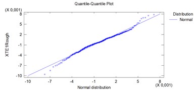
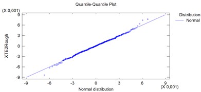
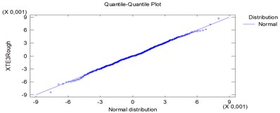
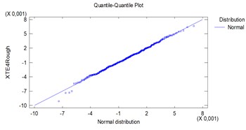
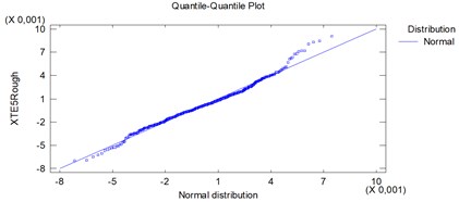
Table 3Polynomial models
Model | R-squared | Standard Error of Estimation |
99.6715 | 0.057317 | |
-10 | 99.5088 | 0.0700857 |
99.2819 | 0.0847431 | |
99.703 | 0.0544984 | |
98.2644 | 0.131743 |
The output at Table 3, shows the results of fitting a seventh order polynomial model to describe the relationship between variables (Fig. 3). The adjusted R-squared statistic, which is more suitable for comparing models with different numbers of independent variables, indicates that the model as fitted explains more than 98 % variability of independent variable. The standard error of the est. value can be used to construct prediction limits for new observations. The P value at each models, analysis of variance, is less than 0.05, there is a statistically significant relationship between the dependent and the independent variables at the 95 % confidence level, [11]. All independent variables , 1, 2, 3, 4, 5 are linear transformations of the initial data .
As a result we archive the plots of fitted models for tested 70 meter tram road, presented in Fig. 5.
Fig. 5Plots of fitted models for 5 passes. The units on the vertical axis are centimeters and on the horizontal axis are meters
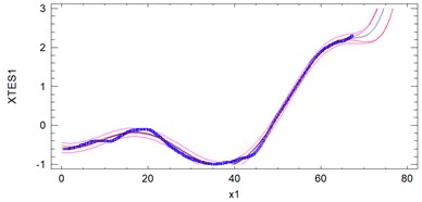
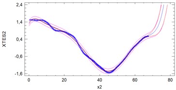
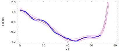
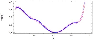
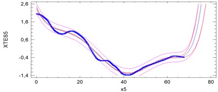
Samples 2, 3, 4 and 5 are rather high compatible. Most outlier sample is first. Sample 5 is characterized by a relatively high instantaneous variability. Analyses show significant deformation of the tram track on the 40 meter test section amounting to 1.4-1.6 cm from its axis. The studies demonstrate the ability to use analysis of positional signals of GPS/Glonass in the maintenance of the network infrastructure of tracks.
4. Conclusions
The use of GLONASS in addition to GPS provides significant advantages in geodesy. The availability of the two-system receiver increases number of satellite signal observations, especially in urban areas, where buildings obscure the signal, reduce the errors significantly affecting the accuracy of positioning and decrease time of GNSS (Global Navigation Satellite System) measurements. The studies confirmed usefulness of wave processing methods for tramp road deformation detection, based on satellite geodesy measurement techniques with high position frequency rate (20 Hz).
The statistical analysis shows that Cross Track Error – XTE can be modeled as a sum of two components: irregular and trend-cycle. The approximation analyzes show that the disorders described by XTER variables are the result of vibrations caused by the measuring equipment as an effect of tram movement. The vibration phenomena in means of transport have been studying in many publications, i.e. [12]. The estimation function of XTES is a weighted average of the functions, where the weights are proportional to the error estimation.
References
-
Global Positioning System Standard Positioning Service Performance Standard. 4th Edition, United States of America Department of Defense, 2008.
-
William J. Global Positioning System (GPS), Standard Positioning Service (SPS) Performance Analysis Report. Federal Aviation Administration, Washington, DC, January 31, 2012.
-
Recommended Standards for Network Transport of RTCM via Internet Protocol (NTRIP). Version 1.0, RTCM Paper 200-2004/SC104-STD, 2004.9.
-
Koc W., Specht C. Results of railway track’s satellite measurements. Technika Transportu Szynowego, Vol. 7-8, 2009, (in Polish).
-
Koc W., Specht C., Jurkowska A., Chrostowski P., Nowak A., Lewiński L., Bornowski M. Determining of railway route course on the basis of satellite measurements. Conference on Designing, Building and Maintenance of Infrastructure in Rail Transportation, Zakopane, Poland, 2009, (in Polish).
-
Koc W., Specht C. Application of the Polish active GNSS geodetic network for surveying and design of the railroad. First International Conference on Road and Rail Infrastructure, Railway Maintenance Section, Opatija, Croatia, 2010.
-
Revnivykh S. 4-th GLObal Navigation Satellite System (GLONASS). Meeting of International Committee on GNSS, St-Petersburg, The Russian Federation, 2009.
-
Department of Defense World Geodetic System 1984, Its Definition and Relationships with Local Geodetic Systems. Technical Report TR8350.2, third edition, 2000.
-
Boashash B. Time-Frequency Signal Analysis and Processing: A Comprehensive Reference. Elsevier Science, Oxford, 2003.
-
Freedman D. Statistical Models: Theory and Practice. Cambridge University Press, 2005.
-
Shumway R. H. Applied statistical time series analysis. Englewood Cliffs, NJ: Prentice Hall, 1988.
-
Burdzik R. Implementation of multidimensional identification of signal characteristics in the analysis of vibration properties of an automotive vehicle’s floor panel. Maintenance and Reliability, Vol. 16, Issue 3, 2014, p. 439-445.
-
Bosy J., Graszka W., Leonczyk M. ASG-EUPOS the Polish contribution to the EUPOS project. Symposium on Global Navigation Satellite Systems, Berlin, 2008.
-
Cord-Hinrich J. SAPOS-part of a geosensors network. Symposium on Global Navigation Satellite Systems, Berlin, 2008.
-
Merrigan M. J., Swift E. R., Wong R. F., Saffel J. T. A refinement to the world geodetic system 1984 reference frame. Proceedings of ION GPS 2002, Portland, 2002, p. 1519-1529.
-
Recommended Standards for Differential GNSS (Global Navigation Satellite Systems) Service. Version 3.0, RTCM Paper 30-2004/SC104-STD, 2004.
About this article

