Analytical research of steel rope dynamic properties

1. Introduction

Diagnostics of steel ropes is a vast area of technical activity; increasing amount of technical installations with ropes raises new tasks for their technical maintenance and early defect finding. Diagnostics of rope covers many fields, for example diameter diminishing, kinematic defects and many others, which has got well developed methods of control and equipment for such control. Nevertheless, broken wires in the rope and their localization along the rope length still beg for improvement of methods, otherwise this work is performed manually.

Finding of broken wires of steel rope surface by electromagnetic methods is still problematic due to the complexity of rope design; these methods are perfect on solid bodies with some irregularities.

Dynamic method of finding of broken wires in the rope [1, 2] brings another opportunity for its diagnostics.

It is necessary to state, that rope consists of many wires, so one broken wire brings very little influence to the stiffness of the whole rope and natural frequency of system.

2. Initial assumptions

Method is realized with fragment of rope, which is fixed at the ends and loaded axially 90 % of its nominal strength. This fragment or rope is excited transversely to rope axis using vibrator, which performs harmonic vibrations.

Few assumptions are necessary to build theoretical model of rope fragment. Size of wire is significantly smaller in size in comparison with the rope. Natural frequency of broken wire relatively to rope body is much higher than the whole rope fragment resonant transverse and rotational vibrations. These statements are quite obvious and are proven by experimental research [3, 4]. In this case vibrations of broken wire and whole rope can be approximately analyzed independently. Thus, by exciting axially loaded rope transverse lowest resonant vibrations, it is possible to state that broken wire elastic deformations are small and can be neglected. Wire is excited through rope body cinematically through attachment point; nevertheless, model in the paper covers vibrations of rope body itself. Problem of broken wire vibration is solved using rotational form of rope vibration as sufficient condition for proposed method application [5-8].

From [9-11] and experimental experience is known, that axial tension of rope creates the twist of the rope. Therefore transversal vibrations of rope create rotational ones, exciting them parametrically. Parametrical vibrations have two time higher frequency than transversal ones. An effort is made to build a model of rope, which will evaluate transverse and rotational vibrations of rope and will enable simple modelling of rope without solving complex and heavyweight contact and friction problem like in case of the final element analysis.

3. Theory

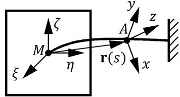
Model of rope fragment was built as lumped mass model of massless string, with equal masses m were attached to string equally spaced by distance $a$, as shown in Fig. 1. String is assumed to have stiffness in axial direction, bending and rotational directions. Tension of string will create twisting of neighboring mass.

Fig. 1Lumped mass model of rope fragment

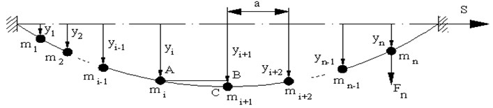
Rope is excited harmonically by force $F_n=F\mathrm{s}\mathrm{i}\mathrm{n}\upsilon t$, applied to $n$th lumped mass. Position of vibrating rope fragment is defined by $n$ generalized coordinates:

In this model it is assumed that rope is vibrating in vertical (drawing) plane. Equations of movement of this model will be derived using Lagrange’s equation of the second kind:

where $T\text{,}$$\mathrm{\Pi }$ – kinetic and potential energy of researched system, $\mathrm{\Phi }$ – dissipative function, $Q_i$ – generalized force applied to coordinate ${\dot{y}}_i$.

Expressions of potential energy are built using methodology [12].

In such model every fragment of string is modelled as beam, fixed in one end and attached to solid body $S$ with coordinate system $M\xi \eta \zeta$, as shown in Fig. 2.

Fig. 2Coordinate system of elastic beam as massless string component

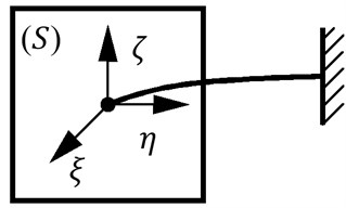
Fig. 3Coordinate system of solid body after small displacement and deviation

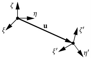
In case of linear displacement $\mathbf{u}$ and deviation $\mathbf{\theta }$ are applied to solid body $S$, coordinate system axis will occupy new position $M\text{'}\xi \text{'}\eta \text{'}\zeta \text{'}$, as represented in Fig. 3.

It is assumed that displacement and deviations are small. Then, projections of vector $\mathbf{u}$ and axis $u_{\xi }$, $v_{\eta }$, $w_{\zeta }$ and deviation angles $M\xi$, $M\eta$, $M\zeta$ of coordinate system $M\xi \eta \zeta$ is assumed to be generalized coordinates.

Every coordinate corresponds to elastic reactions, which consists of main vector ${\mathbf{V}}^0$ and reactions of elastic beams to main moment ${\mathbf{L}}^0$ projections to axis $M\xi \eta \zeta$ is $V_{\xi }^0$, $V_{\eta }^0$, $V_{\zeta }^0$, $L_{\xi }^0$, $L_{\eta }^0$, $L_{\zeta }^0$, where –${\mathbf{V}}^0$ and –${\mathbf{L}}^0$ – main force vector and main force moment vector correspondingly, applied in cross-section $M$, assumed to be applied slowly and slowly restored to equilibrium.

When in point $A$ on beam applied main force vector –$\mathbf{V}$ and main force moment vector –$\mathbf{L}$, beam part $MA$ will remain in equilibrium, when force –${\mathbf{V}}^0$and moment –${\mathbf{L}}^0$ applied in cross section $M$ and force $\mathbf{V}$ and moment $\mathbf{L}$ applied in cross section $A$, as shown in Fig. 4.

Equilibrium equation regarding point $M$ is:

or:

where: $\mathbf{r}\left(s\right)$ – radius-vector of beam axis with ort in point $M$; $s$ – is the arc of $MA$, calculated along the beam axis.

Projections of vector $\mathbf{r}\left(s\right)$ to axis $M\xi \eta \zeta$: $\xi \left(s\right)$, $\eta \left(s\right)$, $\zeta \left(s\right)$.

After evaluation of these statements and assuming Eq. (3), these equations are given:

Projections of vector $\mathbf{L}$ to axis of coordinate system $Axyz$ is represented in Fig. 5.

Fig. 4Equilibrium condition in the beam

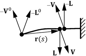
Fig. 5Projections of vector L to axis of coordinate system Axyz

Projections of vector $\mathbf{L}$ to axis of coordinate system $Axyz$ are bending moments $L_x$, $L_y$ and torque $L_z$:

where: $\alpha =\left|\begin{array}{lll}{\alpha }_{11}& {\alpha }_{12}& {\alpha }_{13}\\ {\alpha }_{21}& {\alpha }_{22}& {\alpha }_{23}\\ {\alpha }_{31}& {\alpha }_{32}& {\alpha }_{33}\end{array}\right|$ – matrix of cosines.

In general case potential energy of beam is:

where $A$ and $B$ – are bending stiffness coefficients, $C$ – is the torque stiffness, $l$ – is the length of the beam.

Here it is assumed that modelled rope is strait and rope twisting from its deviation is evaluated by inclination angle from axis $\xi$. Also it is assumed that axis of rope remains in the plain, as explained in Fig. 6.

Then equation of beam axis will have a form:

Then matrix of cosines will be:

Equations, describing beam bending, in case of beam axis inclination and its point leaving plane $M\xi \eta$ will develop torque. This can be evaluated as:

where $V_{\zeta }^0=F_{\zeta }$, $L_{\xi }^0=M_{\xi }$, $L_{\eta }^0=M_{\eta }$.

Then potential energy will be:

Coefficients $C$ and $B$ are obtained experimentally.

After reordering and differentiation according $F_{\zeta }$, $M_{\xi }$ and $M_{\eta }$, matrix of flexibility is given:

where $l=\text{0}\text{.}\text{16875}$ – length of researched rope fragment; $H_S=\eta \mathrm{\text{'}}{\left(s\right)}^{\mathrm{\text{'}}}=\text{0.01}$; $C=\mathrm{}$0.1485 N⋅m²; $B=E{I}_y=\mathrm{}$54.626 N⋅m².

Generally matrix of stiffness: $\left[c\right]={\left[{\beta }_{flex.}\right]}^{-1}$.

In this case potential energy can be expressed as:

Fig. 6Deviation of rope axis in the plane

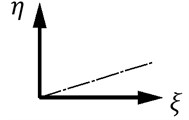
Fig. 7Beam, as component of rope model

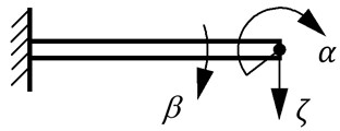
Active coordinates of beam as component to the rope are presented in Fig. 7.

This beam will represent properties of rope and complex rope design then simply represented by such beam within prescribed paradigm.

4. Building of rope model

Dynamic model of rope fragment is built from the previously described beams as discrete elements. Model itself and live coordinates are presented in Fig. 8. As initially decided, model consists from 7 elements; therefore all matrixes have range 7.

Fig. 8Model of rope fragment

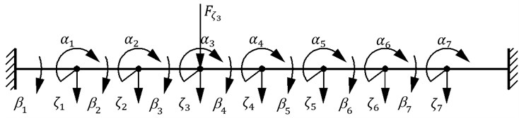
By defining potential energy of one element and evaluating differences of coordinates, the potential energy of all system is built. By differentiating it according generalized coordinates $\left\{q\right\}={\left\{{\zeta }_1,{\alpha }_1,{\beta }_1,{\zeta }_2,{\alpha }_2,{\beta }_2,\dots ,{\zeta }_7,{\alpha }_7,{\beta }_7\right\}}^T$, general matrix of stiffness ${\left[c\right]}_{common}$ is obtained.

While process of damping here is just evaluated, it is assumed that damping matrix is proportional to matrix of stiffness, i.e. $\left[B_{damp.}\right]=\gamma \left[c_{common}\right]$.

Where $\gamma =\text{0.0001}$ and this well corresponds to the experimental research.

Matrix of inertia consists only from elements in main diagonal Eq. (13):

All masses of elements are equal and real value of them:

Moments of inertia are also equal:

Moments of bending $I_{{\beta }_1}=I_{{\beta }_2}=I_{{\beta }_3}=I_{{\beta }_4}=I_{{\beta }_5}=I_{{\beta }_6}=I_{{\beta }_7}=\mathrm{}$7.8168e-5 kg⋅m².

Differential equations of whole rope fragment model is described in form as:

Model is excited by transverse time dependent force, applied to 3rd lumped mass; therefore generalized forces are given in the form:

where only $F_{{\zeta }_3}$ is presented in the load vector. This form of input is directly used in the program [13].

5. Solution and results of rope model

System of differential equations of model was solved numerically using MatLab module Simulink. By implementing operator of differentiating $p=d/dt$ equations were transformed into operator form.

This Eq. (16) is used to build such Simulink model and allows even enter more nonlinearities in the model, for example, nonlinear damping:

Using methodology of [13], Simulink model was build. This model is universal and to any input from available ones is possible to add excitation as force or moment.

In our case input for such system is sine wave, applied to 3rd mass as transverse force; therefore it corresponds to the conditions of experimental research and allows comparing these results. Below in Fig. 11, in photo of experimental setup, a mini exciter is seen, placed directly in the position on the rope, which corresponds to position or 3rd lumped mass on theoretical model, shown in Fig. 8.

Solution in form of amplitude-frequency characteristic in dimensionless form delivers resonant frequencies. These characteristics are graphically presented in Fig. 9. Performing further results analysis, it is noticed, that first and second peak – 70 Hz and 130 Hz represent transverse vibrations, 3rd peak – 192 Hz corresponds to rotational form of vibrations. Nevertheless, all values of this characteristic on the graph represent rotational shape of vibration. Values of rotational vibration amplitude, presented in Fig. 9, are expressed in radians.

Fig. 9Resulting amplitude-frequency characteristics (rotational coordinate α3)

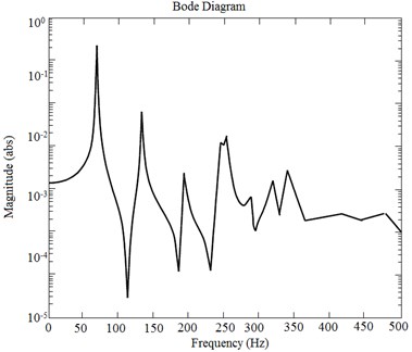
Fig. 10Resulting amplitude-frequency characteristics for ζ3 as transverse vibration

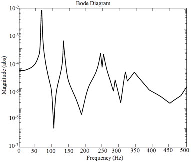
In case of analysis when only rotational form of vibrations is in the scope, result of variables ${\alpha }_1$, ${\alpha }_2$, …, ${\alpha }_7$ gives the answer. Higher shapes of vibrations here are not covered and neglected, as they have no practical value. Higher frequency vibrations have tiny amplitudes (order of micrometers) and measurement of them in real equipment is costly and hardly applicable. First rotational vibration shape at 192 Hz brings over 10 time’s bigger amplitude of response to excitation amplitude, for such measurement requires simple enough equipment.

Pure transverse vibration as output of $\zeta$ is presented in Fig. 10. There is no 3rd peak, representing pure rotational shape of vibration.

Practical implementation of rope model for definition of desired vibration shape frequency is based on obtaining of clear rotational vibration shape. In case of some extra masses or inertia moments on rope (grease, dirt, special marks, etc.), it should be evaluated by input of these in the initial data.

Experimental research was performed using 4 mm rope (5), which was clamped in holders (2) and (7) and tensed with 300 N axial forces. Electrodynamics mini exciter 4810 (6) is tightly clamped to frame (1) and to rope (5) (Fig. 11).

Fig. 11Test rig vibration measuring diagram: 1 – test rig body; 2 – rope support; 3 – linear displacement transducer “Hottinger Tr4”; 5 – linear displacement transducer “Hottinger Tr102”; 5 – tested rope; 6 – electro dynamic mini exciter type 4810; 7 – rope support; 8 – exciter amplifier 2706; 9 – amplifier “Hottiger KWS 503 D”; 10 – generator for electro dynamic mini exciter type 1027; 11 – computer

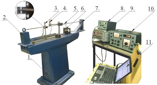
Electrodynamics mini exciter 4810 (6) is fed through amplifier 2706 (8) from generator. Vibration of rope and rope broken wire is measured by linear displacement transducer “Hottiger Tr102” (4), which is fixed in holder of sensor Tr102. Vibration of broken wire was measured by linear displacement sensor “Hottiger Tr4” (3), which was fixed in holder of sensor Tr4. Signals of displacement sensors (4) and (3) through amplifier “Hottiger KWS 503 D” (9) were transmitted to processing centre 9727 driven by computer (11).

Fig. 12Experimentally defined amplitude-frequency characteristics of rope fragment with the same physical parameters

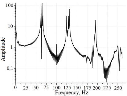
Amplitude-frequency characteristics, obtained during experimental research, are presented in Fig. 12. Peaks in the presented graph, are placed in the same order, first peak – 64 Hz, second peak 130 Hz. Two first peaks represent transverse vibrations and this is detected by measurements. Third peak with frequency 193 Hz represent rotational vibration, sensors detected vibration in transverse vibration shape, too. Experimentally obtained results are important, that resonant frequencies shown in the Fig. 12 corresponds to theoretically prescribed results. Each shape of rope vibration – rotational, transverse is important as dynamic response to parametric excitation, nevertheless only rotational vibration shape is important for broken rope wire detection and here it is evidently presented and corresponds to 3rd resonant frequency. There should be added that in all vibration shapes transverse vibration is present, i.e. no pure rotational shape available here, but for practical measurements in 3rd shape transversal component is neglected.

Good correspondence of frequency between theoretical and experimental research results brings possibility of implementation of presented methodology of modelling.

Method detection of broken wire in the rope uses excitation of rotational shape of tensed steel rope using transverse excitation by vibrator. Presented material in the paper proves theoretically and experimentally, that it is possible to excite rotational vibration of rope in the technical equipment, where access for rotational equipment is technically not possible. Detection of broken wire itself based on use of contactless sensors able to detect vibration of free wire ending, placed distantly from rope surface.

6. Concluding remarks

Performed analysis of rope fragment as simplified lumped mass model with specific behavior allows drawing some conclusions:

1. Good coincidence of theoretical and analytical solution demonstrates adequacy of chosen theoretical model.

2. Comparison of analytical obtained and experimentally measured resonant frequencies brings quite good coincidence on first 3 frequencies (8 %).

3. Created methodology can be easily implemented for different size and design rope behavior modelling and requires simply define two static characteristics experimentally.