Abstract
The 2008 Wenchuan earthquake in China induced many landslides. Gigantic slope failures have attracted serious concerns in engineering practice; however, small slope failures should also be investigated as they are more common. In particular, the detailed characteristics of slope failures during earthquakes remain unknown. Therefore, the present study carried out 1-G shaking table tests on a straight shape slope model with different shaking intensities and frequencies. The test results showed the amplification of motion, the initiation of failure, and final failure mode of the straight shape slope. Also, the experimental results can be used to investigate the response and amplification behavior of some prototype slopes. The results are helpful to demonstrate the detailed collapsing behavior of the slope under earthquake excitation, and provide useful data to analyze the failure mechanism of landslides and valuable references for seismic design of landslide engineering.
1. Introduction
Seismic landslide is one of the main disasters caused by earthquakes [1-4]. The 2008 Wenchuan earthquake (8.0) in Sichuan Province of China induced approximately 20,000 slope failures [5], among which the large earthquakes have drawn engineering attention because they killed many people and formed natural dams, further leading to the risk of breaching and flooding [6-8].
At present, analysis and prediction of seismic landslide basically include three aspects, namely remote sensing techniques, analog methods, theoretical analysis and experimental modeling. The remote sensing technique is used to study an area before and after the occurrence of earthquake using panchromatic sharpened linear imaging self scanning images, in which landslide inventories are first produced. Thus the remote sensing technique is an appraisal procedure, rather than predicting the probability of a landslide occurrence. The analog method is used mainly to predict the occurrence probability of a landslide under potential earthquake by comparing with previous landslides in typical earthquakes. Therefore, the analog methods is only an empirical method. The method of theoretical analysis focuses on the mechanical behaviors under earthquake using analytical or numerical methods. However, it is difficult to describe the complex behaviors in the process of a landslide, and the parameters of rock mass, which are needed in numerical simulation, can only be determined approximately. Experimental modeling can well reflect the occurrence mechanism and process of a landslide under earthquake at the model scale and the manner of exerting seismic loading is suitable.
In this regard, the present paper focuses on failures of relatively small scale slopes which occur much more often than the large ones. The present study determines the initiation of the earthquake-induced landslide with approaches based on either the acceleration of the sliding body or the development of displacement. Further, the effects of nonlinear stress-strain characteristics of soils are considered. This is because the shallow part of mountain slopes is often subjected to weathering and hence is composed of fragmentary rocks. As a result, an elastic dynamic analysis is merely an oversimplified approach for design, and nonlinear dynamic response and failure behavior of mountain slopes should be further studied. It is noteworthy that many mountain slopes once subjected to strong earthquakes became instable in later earthquakes, with features such as debris flow [9-13]. This confirms the importance of considering mountain slopes as consisting of soils rather than intact rocks.
To more realistically demonstrate the behavior of small scale slopes, the present study was undertaken by performing 1-G shaking table tests on models of mountain slopes undergoing different intensities and frequencies of shaking.
2. Landslide model for shaking table tests
2.1. Prototype slope
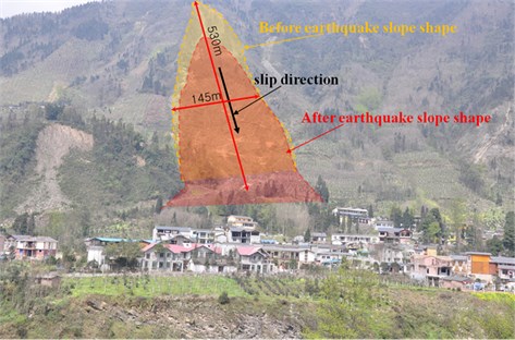
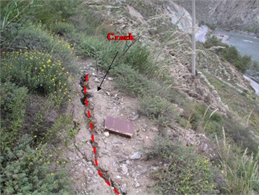
Fig. 1 illustrates a slope failure of relatively small size that occurred at Tazhiping in Dujiangyan City at the location (103.375_E, 31.629_N) in the Hongse village, Hongkou Town. It is evident that the slip plane is rather straight, suggesting that the weak materials at the surface fell under seismic excitation. There were many similar events associated with straight slip planes in the Wenchuan earthquake-hit region. The Tazhiping landslide was triggered by the main shock of Wenchuan earthquake and caused at least 1 fatality. The elevation of the landslide ranged from 1107 m to 1370 m. Its length was about 530 m, and the width was about 145 m. The landslide lithology was fragmentary rocks and the surface was covered by silty clay and gravel. The space distribution of slippery bodies was thick in the center and thin near the perimeter, and the estimated thickness of the sliding mass was 20 m to 25 m. The estimated volume of the landslide was about 116×104 m3. The landslide angle was around 32 degrees.
Fig. 1The Tazhiping landslide
To investigate the deformations and failure mechanisms of straight slopes, a series of tests was performed with different input amplitudes and frequencies of sinusoidal waves. Based on the measurements of the acceleration and displacement of different points in the slope model, the dynamic characteristics and responses of the straight model slope under earthquake, as well as the influence of ground motion parameters, are discussed.
2.2. Test set-up and instrumentation
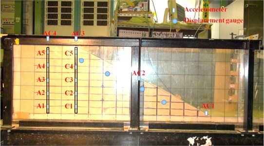
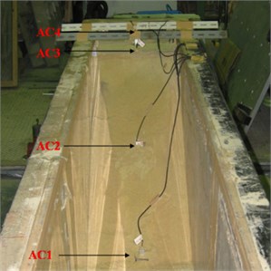
The shaking table at the Geotechnical Engineering Laboratory, University of Tokyo, is 2 m wide and 3 m long, and is capable of applying bi-directional horizontal accelerations. The bearing capacity of the shaking table is 7 tons, and the maximum applied acceleration is 1,000 Gal (≈1 g) frequencies up to 50 Hz. Soil slope models were prepared in a soil container with 3 m in length, 0.4 m in width and 0.6 m in depth. This container was tightly fixed onto the shaking table so that there was no slippage between them. A total number of 14 accelerometers and 4 displacement gauges were installed to measure horizontal dynamic responses during the experiments (inclinometers were prepared by making a column of accelerometers) [14-16]. Fig. 2 shows that the accelerometers were installed in vertical arrays below the crest and the shoulder as well as along the slope to measure the distribution of accelerations inside the slope model. It is also seen that square grids with color were installed in the vertical glass wall to demonstrate visually the dynamically-induced deformation of the model.
Fig. 2Slope model with accelerometers and displacement gauges
2.3. Slope models in testing
Slope models consisted of uniform Toyoura sand with the mean grain size of 0.174 mm and the void ratio between 0.605 and 0.974. In the preparation of the slope models, the relative density of 32 %, the void ratio of 0.857, and the moisture content of 1 % were used. The effective stress in the small-scale 1-G model tests was around 1/500 of the prototype, and thus the density of sand was reduced so that similitude of dilatancy was maintained [17-19]. In line with this, the time scale in the model tests was made shorter than the prototype event in consideration of the reduced size of models by shaking all the models at, for example, 10 Hz, which was higher than the real earthquake events. Shaking at lower frequencies of 2 and 5 Hz was run as well. The duration of shaking was 30 seconds. The moisture content of 1 % was employed to provide a certain apparent cohesion to the sand to avoid failure at the very surface of the slope. The intensity of base shaking in the horizontal and longitudinal direction of models varied from 100 to 700 Gal.
3. Dynamic responses and failure of straight-slope model
3.1. Dynamic responses
Fig. 3 shows the dimensions of the straight-slope model. As in the aforementioned Tazhiping case, the slope angle of the model was 32 degrees.
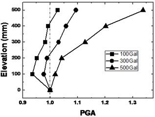
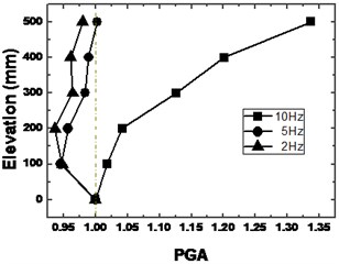
Fig. 4 shows detailed acceleration time histories. Fig. 5 plots the ratio of maximum acceleration (amplitude) along the vertical array in the slope (A1 to A5 in Fig. 2) to the shaking table acceleration. The case of 500 Gal shaking under frequency of 10 Hz exhibits more remarkable amplification than others, as shown in Fig. 5(a). This is most probably due to the nonlinear stress-strain behavior of sand in that the elastic modulus decreases as the dynamic stress and shear strain increase, leading to varying natural periods in the model. This point is examined in more detail in Fig. 5(b), in which the variation of amplification with shaking frequency is plotted for base acceleration with input seismic wave of 500 Gal. Fig. 5(b) shows that the case of 10 Hz is probably closer to the resonance frequency of the model, exhibiting more remarkable amplification than the other cases.
Fig. 3The tested model slopes (unit: mm)
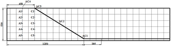
Fig. 4Time histories of acceleration along the slope
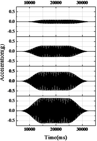
Fig. 5Distribution of acceleration inside a slope model
a) 10 Hz excitation
b) 500 Gal excitation
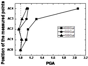
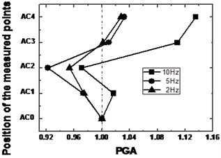
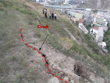
Fig. 6(a) shows the ratio of the maximum acceleration (i.e. amplitude) at the surface of the slope (AC1 to AC4 in Fig. 3) to that applied the base with amplitude up to 500 Gal. This allows study of the effects of nonlinearity of soils in greater detail. Actually, shaking at 700 Gal caused slope failure and thus the corresponding results are not included in Fig. 6. AC4 at the crest shows more significant amplification than the other cases. The amplification at the slope shoulder (AC3) is large as well but smaller than that at the crest (AC3AC4). This is consistent with the findings after the Wenchuan earthquake that many cracks formed in the back scarp of the slope, although the main body of the slope was intact (Fig. 7). Fig. 6(b) illustrates that with increasing height (AC1 to AC4), the acceleration at the slope surface decreases and then increases at the mid-height of the slope.
Fig. 6Distribution of acceleration at the surface of the straight slope model
a) 10 Hz excitation
b) 300 Gal at base
Fig. 7Two cracks in the back scarp of the slope
3.2. Failure modes of straight slope models
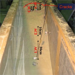
Fig. 8 illustrates the failed shape after 700-Gal shaking at 10 Hz frequency. The square grids in the photo clearly indicate that shear failure or slippage took place at some depth below the surface, as expected by using 1 % moisture content. The linear shape of the shear plane was similar to the failure of the prototype slope as shown in Fig. 1.
Fig. 8Failed straight slope with 32-degree gradient subjected to shaking of 700 Gal and 10 Hz for 30 seconds
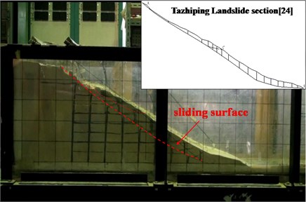
Fig. 9Acceleration response along the surface of a straight slope (32 degrees, 700 Gal, 10 Hz)
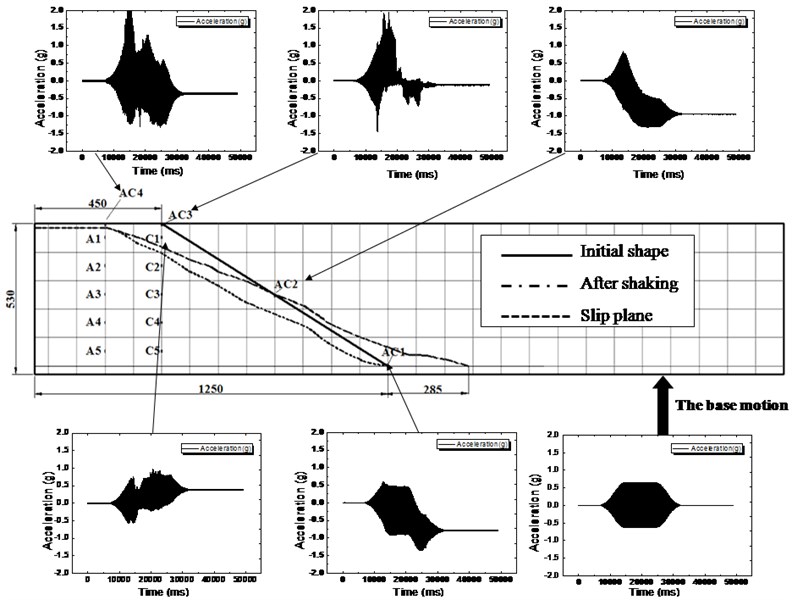
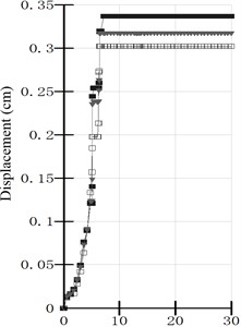
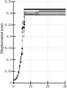
Fig. 10Time history of displacements derived from the measured accelerations
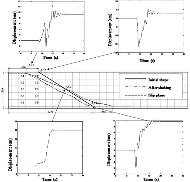
Fig. 9 compares the shape of the slope before and after shaking. The model slope, nearly intact under 500 Gal shaking, suddenly developed cracks and then slid at shallow depth below the slope under 700 Gal shaking. In the same figure, the time histories of horizontal acceleration along the slope surface are shown. The bias from zero is due to tilting of the transducer after slope failure. From the amplitude of acceleration at the slope surface, it is found that the shaking was weaker in the lower part of the slope (AC1 and AC2), and stronger in the upper half (AC3 and AC4). The increasing acceleration towards the top was caused by energy concentration at the narrower slope, as observed in reality. Moreover, the acceleration in the slope shoulder (C1) became less than that at the surface.
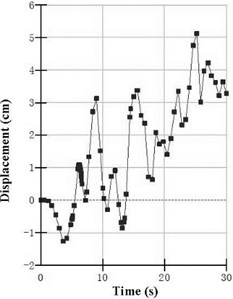
The recorded acceleration was integrated twice and the effects of tilting and other baseline errors from the acceleration were removed to obtain the time history of displacement, as shown in Fig. 10. Clearly, the displacement amplitude, which was closely related to the local shear strain amplitude, increased from the bottom (AC1) to the shoulder (AC3) and the crest of the slope (AC4), indicating more nonlinearity and extent of yielding of soils at higher elevations. The significant shear strain induced large deformation. The failure was initiated at AC4 at the crest and then proceeded to AC1 at the bottom of the slope. Fig. 11 traces the development of slope failure with time. The displacements in this photo are consistent with the findings in Fig. 10.
Fig. 11Development of slope failure
a) Before slope failure
b) After slope failure
3.3. Location and shape of sliding surface
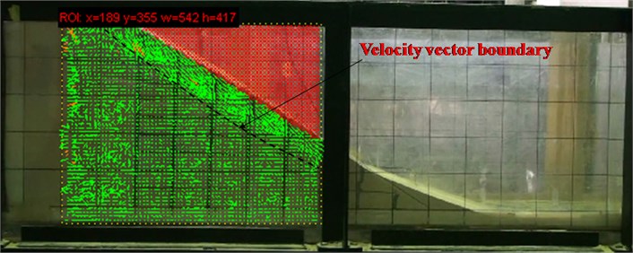
The deformation of the slope subjected to seismic loads was further studied by the particle image velocimetry (PIV) [18]. Fig. 12 presents a digital cross-correlation analysis of double frame/single exposure records, in which the cross-correlation between two interrogation windows sampled from the image records is calculated [20] and the displacement of sand grains between photographs at two time points is detected. The PIV technology was applied to large-scale shaking table model tests of slope stability, and Fig. 13 indicates that the displacement and the velocity were greater above a plane known as the slip plane.
Fig. 12PIV process for tracking displacement vector [15]
![PIV process for tracking displacement vector [15]](https://static-01.extrica.com/articles/15664/15664-img16.jpg)
The results show that the PIV technology could effectively measure the displacement of any point at any time with accuracy within the observation region. Furthermore, more information about the process of deformation development could be obtained, such as the formation of strain localization and the whole failure process of slopes under earthquake.
Fig. 13PIV analysis results with velocity vector boundary of slope
4. Numerical analysis on a straight slope model
To compare the dynamic failure of slope model in shaking table tests, a finite-element dynamic analysis was performed. The total number of elements was 804 with 886 nodes, as shown in Fig. 14. For this analysis, an elastic-perfectly plastic constitutive model with the Mohr-Coulomb failure criterion was adopted for soils. The input parameters for slightly wet Toyoura sand are shown in Table 1 [21]. The sand parameters will be discussed later. 300 Gal (10 Hz) and 700 Gal (10 Hz) seismic wave inputs were applied at the bottom of the numerical model, which was consistent with the shaking model tests (see Fig. 2). The duration of shaking was 30 seconds.
Fig. 14Finite element model of a slope
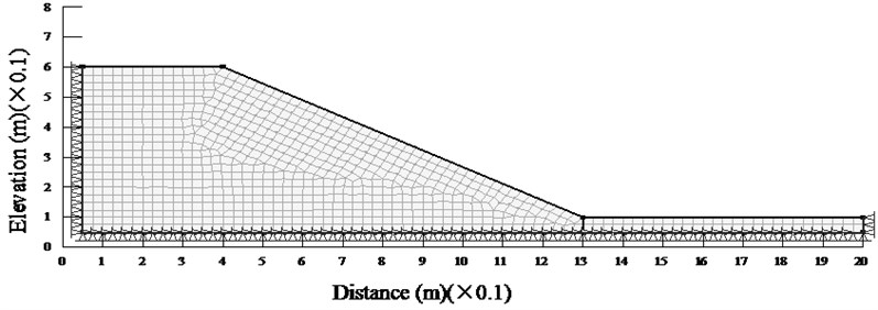
Table 1Parameters of the Toyoura sand
Gravity | Unit weight | Cohesion | Friction angle | Young’s modulus | Poisson’s ratio |
(g/cm3) | (kN/m3) | (kPa) | (°) | (kPa) | |
2.648 | 19.6 | 7.2 | 38 | 6000 | 0.25 |
Fig. 15 shows the peak acceleration within the slope and at its surface (corresponding to AC1-AC4 and A1-A5 in Fig. 1), respectively. Compared with the model tests (Fig. 5(a)), the calculated accelerations under this relatively weak shaking are similar to the experimental findings. Therefore, the FEM approach is suitable for calculating the acceleration in the slope when the whole slope is intact.
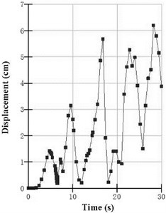
The time histories of the displacement of AC4 and AC3 (as indicated in Fig. 3) are shown in Fig. 16, and correspond to the maximum shear strain in the slope. The displacement at the shoulder of the slope (AC3) is nearly consistent with that from the experiment result (Fig. 11). However, at the crest of the slope (AC4), the calculated displacement is smaller than the experiment result. This implies that the simulation is not suitable for evaluating the failed shape of a slope, because conventional FEM cannot properly deal with large deformation.
Fig. 15Time history of accelerations in the numerical analysis (300 Gal, 10 Hz, a) at the surface of a straight slope (AC1-AC4) and b) within a straight slope (A1-A5))
a)
b)
Fig. 16Time history of displacements in the numerical analysis (700 Gal, 10 Hz, a) at the crest AC4 and b) at the shoulder AC3)
a)
b)
5. Conclusions
A series of shaking table tests was conducted in 1-G environment to study the effects of shallow slope instability during earthquakes. The effects of reduced confining pressure and the small model size as compared with the prototype were taken into account by employing reduced sand density and shortened time scale. The major findings from this study are summarized as follows:
1) Model tests show that greater acceleration developed near the top of the slope, suggesting the amplification of motion. The displacement amplitude, which was closely related to the local strain amplitude, increased from the bottom to the top of the slope, indicating greater nonlinearity and extent of yielding of sand soils at higher elevations.
2) The acceleration near the shoulder of the slope (AC3) was greater than that at the crest of the slope (AC4) when the slope angle was small. This suggests that failure is initiated from the shoulder.
3) The PIV technology was able to effectively measure the displacement of any point at any time with reasonable accuracy within the observation region. Furthermore, more information can be obtained about the process of deformation development, the formation of strain localization and the whole failure process of slope under earthquakes.
4) The FEM approach is suitable for describing the acceleration in the slope when the whole slope is intact. However, the simulation is not suitable for evaluating the failed shape of a slope.
References
-
Pradel D., Smith P. M., Stewart J. P., Raad G. Case history of landslide movement during the northridge earthquake. Journal of Geotechnical and Geoenvironmental Engineering, Vol. 131, Issue 11, 2005, p. 1360-1369.
-
Chigira M., Yagi H. Geological and geomorphological characteristics of landslides triggered by the 2004 mid Niigata prefecture earthquake in Japan. Engineering Geology, Vol. 82, Issue 4, 2006, p. 202-221.
-
Keefer D. K., Wartman J., Ochoa C. N., Rodriguez M. A., Wieczorek G. F. Landslides caused by the M7.6 Tecoman, Mexico earthquake of January 21, 2003. Engineering Geology, Vol. 86, Issue 2-3, 2006, p. 183-197.
-
Qiao J. P., Huang D., Yang Z. J. Discussion on macro-epicenter of Wenchuan earthquake. Journal of Catastrophology, Vol. 28, Issue 1, 2013, p. 1-5, (in Chinese).
-
Yin Y. P., Wang F. W., Sun P. Landslide hazards triggered by the 2008 Wenchuan earthquake, Sichuan, China. Landslides, Vol. 6, Issue 2, 2009, p. 139-151.
-
Huang R. Q. Mechanism and geomechanical modes of landslide hazards triggered by Wenchuan 8.0 earthquakes. Chinese Journal of Rock Mechanics and Engineering, Vol. 28, Issue 6, 2009, p. 1239-1248, (in Chinese).
-
Wang F. W., Cheng Q. G., Lynn H. Preliminary investigation of some large landslides triggered by the 2008 Wenchuan earthquake, Sichuan province, China. Landslides, Vol. 6, Issue 6, 2009, p. 47-54.
-
Huang R. Q. Analysis of the geo-hazards triggered by the 12 May 2008 Wenchuan earthquake, China. Bulletin of Engineering Geology and the Environment, Vol. 68, Issue 3, 2009, p. 363-371.
-
Pareek N., Pal S., Mukat L. S., Manoj K. A. Study of effect of seismic displacements on Landslide Susceptibility Zonation (LSZ) in Garhwal Himalayan Region of India using GIS and remote sensing techniques. Computers and Geosciences, Vol. 61, 2013, p. 50-63.
-
Lee C. T. Statistical seismic landslide hazard analysis: an example from Taiwan. Engineering Geology, Vol. 182, 2014, p. 201-212.
-
Gokhan S., Ellen M. R. Probabilistically based seismic landslide hazard maps: an application in Southern California. Engineering Geology, Vol. 109, Issues 3-4, 2009, p. 183-194.
-
Randall W. J., Edwin L. H., John A. M. Method for producing digital probabilistic seismic landslide hazard maps. Engineering Geology, Vol. 58, Issues 3-4, 2000, p. 271-289.
-
Rajabi A. M., Khamehchiyan M., Mahdavifar M. R., Gaudio V. D., Capolongo D. A time probabilistic approach to seismic landslide hazard estimates in Iran. Soil Dynamics and Earthquake Engineering, Vol. 48, 2013, p. 25-34.
-
Zhou X. P., Cheng H. Stability analysis of three-dimensional seismic landslides using the rigorous limit equilibrium method. Engineering Geology, Vol. 174, 2014, p. 87-102.
-
Lenti L., Martino S. The interaction of seismic waves with step-like slopes and its influence on landslide movements. Engineering Geology, Vol. 126, 2012, p. 19-36.
-
Wu J. H. Seismic landslide simulations in discontinuous deformation analysis. Computers and Geotechnics, Vol. 37, Issue 5, 2010, p. 594-601.
-
Wang K. L., Lin M. L. Seismic slope behavior in a large-scale shaking table model test. Engineering Geology, Vol. 82, Issue 4, 2006, p. 202-221.
-
Wang K. L., Lin M. L. Initiation and displacement of landslide induced by earthquake-a study of shaking table model slope test. Engineering Geology, Vol. 122, Issue 4, 2011, p. 106-114.
-
Liu J., Liu F. H., Kong X. J., Li Y. S. Application of PIV in large-scale shaking table model tests. Chinese Journal of Geotechnical Engineering, Vol. 32, Issue 3, 2010, p. 368-374, (in Chinese).
-
Towhata I., Jiang Y. J. Special Topics in Earthquake Geotechnical Engineering. Springer Netherlands, Germany, 2010.
-
Sendir T. S., Sato J., Towhata I., Honda T. 1-G model tests and hollow cylindrical torsional shear experiments on seismic residual displacements of fill dams from the viewpoint of seismic performance-based design. Soil Dynamics and Earthquake Engineering Journal, Vol. 30, Issue 6, p. 423-437.
About this article

The present study was conducted within a framework of an international collaboration project between Institute of Mountain Hazard and Environment Chinese Academy of Science and University of Tokyo. This work was supported by National Natural Science Foundation of China (Grant No. 41301009) and the International Cooperation Program of the Ministry of Science and Technology of China (Grant No. 2013DFA21720), the National Science and Technology Support Program during the Twelfth Five-Year Plan Period (Grant No. 2011BAK12B01) and the Guizhou Province Outstanding Young Scientific Talents Training Program Funded Projects (No. (2013) 30). The authors express their gratitude for those aids and assistances.
