Marine propulsion shaft system fault diagnosis method based on partly ensemble empirical mode decomposition and SVM

1. Introduction

By reducing costs and decreasing the repair time, condition based maintenance becomes an efficient strategy for ship industry [1]. Marine propulsion shaft system is the key components of the ship power system. It influences directly the operation of the whole ship. Therefore, it is significant to be able to accurately and automatically detect and diagnose the existence and severity of the faults occurring in the marine propulsion shaft system. Since vibration signals carry a great deal of information representing mechanical equipment health conditions, the vibration based signal processing technique is one of the principal tools for diagnosing bearing faults [2, 3].

Typically, a fault diagnosis system contains two steps. The first step is to extract fault features by signal processing; the second step is to diagnose the faults by the characteristic information obtained in the first step. With the signal processing techniques, faulty characteristic information can be extracted from the vibration signals [4]. Considering the nonstationary of the Marine propulsion shaft system, the time frequency analysis methods such as Wavelet Transform (WT) [5, 6] and Empirical Mode Decomposition (EMD) [7] were used for processing the complex signal. EMD method [8] introduced by Huang et al. is an innovative time-series analysis tool in comparison with traditional methods such as Fourier methods, wavelet methods, and empirical orthogonal functions. A nonstationary and nonlinear signal will be decomposed into several Intrinsic Mode Function (IMF) components by sifting process of EMD. The result is a set of nearly orthogonal functions and the number of functions in the set depends on the original signal [9]. One of the primary weaknesses of EMD method is the phenomenon of mode mixing, which is defined as either a single IMF containing different scales signal, or a signal of a similar scale existing in different IMF components. In order to overcome shortcomings of EMD, a noise-assisted data analysis method called Ensemble EMD (EEMD) was proposed in [10] by adding white noise to initial data. The IMFs derived from EEMD, however, would inevitably be polluted by the added noise especially when the number of trials was in appropriate and this can be really true when reconstructing the original signal from the obtained IMFs. Recently, an enhanced EEMD algorithm called Complementary EEMD (CEEMD) was proposed to improve the efficiency of the original noise assisted method by adding noise in pairs with plus and minus signs [11]. However, in EEMD and CEEMD methods, the ensemble process is time-consuming especially when the number of trials is large. Moreover, the IMFs derived from EEMD and CEEMD often include some false and meaningless IMF components and some of them even do not meet the IMF definition conditions. In older to overcome these disadvantages of EEMD and CEEMD, another noise-assisted method Partly Ensemble EMD (PEEMD) is proposed in [12]. PEEMD decomposes a signal in a CEEMD way in the first ith IMFs and then using EMD in the remaining ranks, instead of implementing ensemble and averaging to all IMFs. Hence, PEEMD can reduce the amounts of calculation of CEEMD and improve the accuracy of obtained IMFs greatly.

Generally the vibration signals are obtained from the monitoring mechanical equipment. After the signal decomposed into several IMFs through PEEMD method, the statistical features like energy and kurtosis can be calculated to describe the characteristics of the signal at each frequency band. These statistical features can be utilized in the fault diagnosis directly, but in practice some of the features extracted from experimental data are usually imperfect and redundancy, even incompatible for each other, accordingly bring forth a lot of problems to mechanical fault diagnosis such as high computational complexity, low recognition speed and weak recognition effect. So it is meaningful to investigate the fault diagnosis method using the less attribute values without missing any fault information.

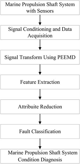
Fig. 1Flow diagram of the proposed fault diagnostic procedure

Principal Component Analysis (PCA) is a well-established method for feature extraction and dimensionality reduction [13]. PCA can be used to represent the d-dimensional data in a lower-dimensional space which will reduce the freedom degrees, the space and time complexities. The objective is to represent data in a space that best expresses the variation in a sum-squared error sense. This technique is mostly useful for segmenting signals from multiple sources. Recently, the principal component analysis has been widely applied in machine fault diagnosis domain [14, 15].

In recent years, SVM has been widely used in many research areas, such as face recognition, signal and image processing and fault diagnosis. SVM based classifiers have better generalization properties than ANN based classifiers [16, 17]. The efficiency of SVM based classifier does not depend on the number of features. This property is very useful in fault diagnostics because the number of features to be chosen is not limited, which make it possible to compute directly using original data without pre-processing them to extract their features. These advantages make SVM an excellent choice for the fault detection and localization applications [18]. Meanwhile, SVM kernel function parameters selection problem is an important factor affecting the performance of classification ability, Genetic Algorithm (GA) was used for optimizing the kernel function parameters.

According to the above principles, a new fault diagnosis method for marine propulsion shaft system is proposed in this paper, which utilizes the PEEMD to extract faulty feature parameters and then makes the attribute reduction in the faulty feature vectors by PCA method to obtain the key features, lastly these key features are input into SVM to accomplish faulty diagnosis. The flow diagram of the presented fault diagnosis method is shown in Fig. 1.

The following of this paper is organized as follows: in Section 2, the statistics parameters of the IMF components are extracted as faulty features by PEEMD. In Section 3, GA-optimized SVM is used to accomplish the fault pattern classification based on the selected features. In Sections 4 and 5, the proposed method is applied to diagnose different conditions of a rolling bearing and stern bearing on marine propulsion shaft system, and the results have verified the validity of the proposed diagnosis method. At last the conclusions have been briefly drawn in Section 6.

2. PEEMD method

By using EMD a complex signal can be decomposed into finite IMFs and a residual item. However, the main problem of EMD is the phenomenon of mode mixing. Aim to this, EEMD is proposed by adding different white noises to the targeted signal. The IMFs derived from EEMD would inevitably be polluted by the added noise. And CEEMD is presented mainly with the aim to decrease the reconstruction error caused by the added white noises. Unlike EEMD, in CEEMD white noises are added in pairs to the original data (i.e. one positive and one negative) to generate two sets of ensemble IMFs. Yet CEEMD and EEMD mainly have the following problems. First, the ensemble process is time-consuming especially when the number of trials is large. Second, the IMFs derived from EEMD and CEEMD often include some false and meaningless IMF components and some of them even do not meet the IMF definition conditions. This is mainly caused by the fact that different noise-added data may generate different number of IMFs, though adding white noise with the same size.

In order to avoid the defects of EEMD and CEEMD, another noise-assisted method partly ensemble EMD is proposed, which decomposes a given signal in a CEEMD way in the first ($j-$1)th IMFs and then using EMD in the remaining ranks, instead of implementing ensemble and averaging to all IMFs. Hence, PEEMD can reduce the amounts of calculation of CEEMD and improve the accuracy of obtained IMFs greatly. PEEMD is described as follows [12, 19].

(1) Suppose $j=$ 1, add white noise series $\left\{n_i\right(t\left)\right\}$ and $\{-n_i(t\left)\right\}$ to the targeted signal $S\left(t\right)$ as:

where $a$ is the amplitude of added white noise, $i=$ 1, 2,…, $N_e$; $N_e$ is the pair number of added white noise. In EEMD Wu and Huang suggested [10] to use small amplitude values for data dominated by high-frequency signals, and vice versa. Hence, they recommended that $N_e$ could be chosen about a few hundred, and the amplitude of added white noise was set about 0.2$SD$, where $SD$ was the standard deviation of the targeted data. The $N_e$ was set 100 and parameter $a$ was set 0.2$SD$ in this paper.

(2) Decompose the two signal series $\left\{r_{ij}^{+}\right(t\left)\right\}$ and $\left\{r_{ij}^{-}\right(t\left)\right\}$ using EMD in the $j$th IMF mode, and two IMF sets $\left\{I_{ij}^{+}\right(t\left)\right\}$ and $\left\{I_{ij}^{-}\right(t\left)\right\}$ can be obtained, as well as two residue sets $\left\{r_{i,j+1}^{+}\right(t\left)\right\}$ and $\left\{r_{i,j+1}^{-}\right(t\left)\right\}$, respectively.

Namely:

(3) Through ensemble the final IMF in the $j$th rank can be derived by:

(4) Calculate the Permutation Entropy (PE) $P_j^{}$ of $I_j^{}\left(t\right)$, if $P_j^{}$ is larger than ${\theta }_0^{}$, then $j=j+$1, and go to steps (2)-(3); if $P_j^{}$ is smaller than ${\theta }_0^{}$, then go to step (5).

As PE is defined to measure the randomicity and dynamic change of time series, according to the experiments in [12], a recommended value of ${\theta }_0^{}$ ranges from 0.5 to 0.6 and in this paper we set ${\theta }_0^{}=$ 0.6.

(5) Separate the first $j-$1 IMFs from the original signal and the residue $r\left(t\right)$ is obtained by:

(6) Decompose $r\left(t\right)$ completely by using EMD:

(7) $\left\{c_k\right(t\left)\right\}$ are regarded as the IMFs following to the first $j-$1 IMFs. The initial signal is informed as:

PEEMD decomposes a given signal in a CEEMD way in the first ($j-$1)th IMFs and then using EMD in the remaining ranks, instead of implementing ensemble and averaging to all IMFs. In order to clarify the decomposition processes, consider the case of the signal as:

The time domain waveforms of $x_1\left(t\right)$, $x_2\left(t\right)$, $n\left(t\right)$ and their mixed signal $x\left(t\right)$ are showed in Fig. 2. The decomposing results of the mixed signal $x\left(t\right)$ are given in Figs. 3-6, respectively.

Fig. 2The time domain waveforms of x1(t), x2(t), n(t) and their mixed signal x(t)

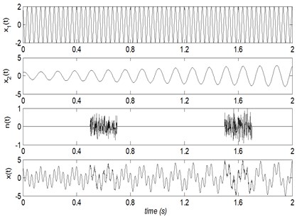
Fig. 3EMD decompose results of the mixed signal x(t)

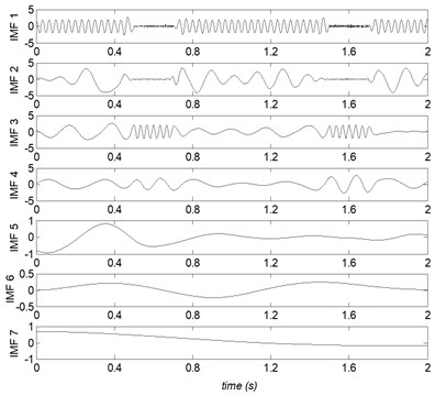
Fig. 4EEMD decompose results of the mixed signal x(t)

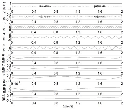
Fig. 5CEEMD decompose results of the mixed signal x(t)

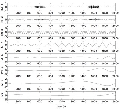
Fig. 6PEEMD decompose results of the mixed signal x(t)

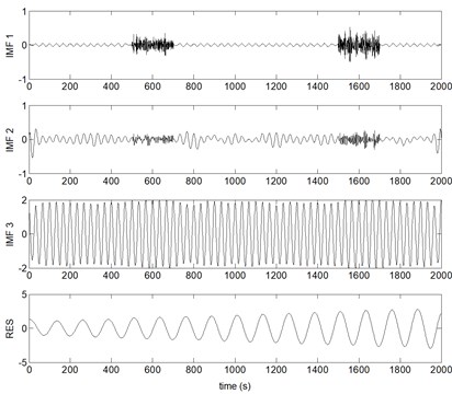
Where IMF $i$ represents the $i$th IMF, and RES stands for the residual, correspondingly. From Figs. 3-6, it can be found that, due to the noise interference, EMD has emerged severe mode mixing and yielded false components without physical meanings. EEMD and CEEMD have similar decomposing results and both of them restrain the phenomenon of mode mixing effectively. The sum component IMF 1 and IMF 2 corresponds to the real component $n\left(t\right)$. However, $x_1\left(t\right)$ and $x_2\left(t\right)$ are divided into seven and five components by EEMD and CEEMD respectively. PEEMD performed well with a zero residue and the components IMF 3 and IMF 4 (RES) are in excellent agreement with the real component $x_1\left(t\right)$ and $x_2\left(t\right)$.

3. SVM method

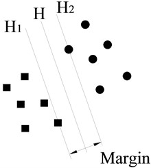
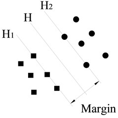
SVM is a statistic machine learning technique proposed by Vapnik [20] and widely used in pattern recognition. Let $\left\{\right(x_i,y_i),i=1,\dots ,N\}$ be a training sample set $Q$ and each sample $x_i$ belongs to a class defined by $y_i\in \left\{-1,\mathrm{}1\right\}$. The goal of SVM is to find a hyperplane which divides $Q$, such that all the points with the same label are on the same side of the hyperplane while maximizing the distance between the two classes I, II and the hyperplane. An example of the optimal hyperplane of two data sets is presented in Fig. 6.

Fig. 7a) A separating plane with small margin and b) a separating plane with larger margin

a)

b)

As shown in Fig. 7, rings and diamonds stand for these two classes of sample points respectively; $H$ is a separating plane. $H_1$ and $H_2$ are planes that are parallel to $H$ and, respectively, pass through the sample points closest to $H$ in these two classes. The distance between $H_1$ and $H_2$ is defined as margin.

For linearly separable data, it is possible to determine a hyperplane that separates the data leaving one class on each side of the hyperplane. This plane can be described by the Eq. (7):

where $w$ is $W\in R^n$ weight vector and $b$ is a scalar. The vector $w$ and the scalar $b$ determine the position of the separating hyperplane. The separating hyper plane should satisfy the constraints:

Positive slack variables ${\xi }_i$ are introduced to measure the distance between the margin and the vectors $x_i$ that lie on the wrong side of the margin. Then, the optimal hyper plane separating the data can be obtained by the following optimization problem:

where $C$ is the error penalty parameter. By introducing the Lagrangian multipliers ${\alpha }_i$, the above-mentioned optimization problem is transformed into the dual quadratic optimization problem, that is:

Thus, the linear decision function is created by solving the dual optimization problem, which is defined as:

SVM can also be used in nonlinear classification by using kernel function. By using the nonlinear mapping function $\mathrm{\Phi }\left(x_i\right)$, the original data $x$ are mapped into a high-dimensional feature space, where the linear classification is possible. Then, the nonlinear decision function is:

where $K(x_i,x_j)$ is called the kernel function, $K(x_i,x_j)=\mathrm{\Phi }\left(x_i\right)\mathrm{\Phi }\left(x_j\right)$.

Any function that satisfies Mercer’s theorem can be used as a kernel function to compute a dot product in feature space. There are different kernel functions used in SVMs, such as linear, polynomial and Gaussian RBF. The selection of the appropriate kernel function is very important, since the kernel defines the feature space in which the training set examples will be classified.

In order to apply SVM in mechanical fault diagnosis, there are two aspects of problems to study. Firstly, we can construct a multi-classifier by combining several binary classifiers for SVM is a binary classification method. Several methods have been proposed, such as ‘one-against-one’ (OAO), ‘one-against-all’ (OAA), and directed acyclic graph SVMs (DAGSVM) [21], where Hsu make a comparison of these methods and point out that the ‘one-against-one’ method is more suitable for practical use than other methods. In this study, we employ ‘one-against-one’ method to diagnose the different faulty condition. Secondly, the radial basis function kernel $K(x_i,x)=\mathrm{e}\mathrm{x}\mathrm{p}(-{‖x_i-x‖}^2/2{\sigma }^2)$ is selected and the Genetic Algorithm (GA) algorithm [22] is adopted for SVM model generalization parameter $\gamma$ selection and searching proper RBF kernel parameter width $\sigma$.

4. Experimental setup and data acquisition

To demonstrate the performance of the proposed fault diagnosis method, two kinds of experimental setups are presented in this section for offering the vibration signals from various faulty conditions of rolling bearings and stern bearing on a marine propulsion shaft system.

4.1. The rolling bearing experiment

The experimental setup consists of a 2 hp motor, a torque transducer, a dynamometer and control electronics. The test bearings support the motor shaft [23]. Motor bearings are seeded with faults using Electro-Discharge Machining (EDM). Faults ranging from 0.007 inches in diameter to 0.040 inches in diameter are introduced separately at the inner raceway, rolling element and outer raceway. Faulted bearings are reinstalled into the test motor and vibration data is recorded for motor loads of 0 to 3 horsepower (motor speeds of 1797 to 1730 RPM). Vibration data is collected using accelerometers, which are attached to the housing with magnetic bases.

Fig. 8Schematic diagram of the propulsion shaft system experiment setup

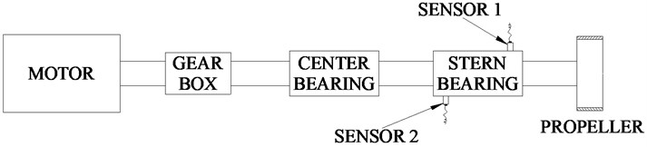
4.2. The propulsion shaft system experiment

The second experiment is to identify different conditions of stern bearing on a propulsion shaft system. As shown in Fig. 8, the test stand consists of a motor, a gear box, a center bearing, a stern bearing and a propeller. The test stern bearing support the propulsion shaft. Several typical faulty conditions of the stern bearing are simulated, such as parallel misalignment being too large and the angular misalignment being too large. Five states including four faulty states and one normal state of stern bearing are tested. The description of the five states of stern bearing is shown in Table 1.

Table 1Five states of stern bearing on propulsion shaft system

Condition code	Faulty description
C-1	Normal condition
C-2	Parallel horizontal misalignment being too large	Horizontal offset 2.5 mm
C-3	Parallel vertical misalignment being too large	Vertical offset 2.5 mm
C-4	Angular horizontal misalignment being too large	The aft of bearing horizontal offset 3 mm
C-5	Angular vertical misalignment being too large	The aft of bearing vertical offset 3 mm

The diameter of the stern bearing is 250 mm. In order to avoid the misalignment is too large which will destroy the propulsion shaft system or too small which will affect the test of faulty conditions, the parallel horizontal misalignment and parallel vertical misalignment are both set 2.5 mm. At the same time, the angular horizontal misalignment and angular vertical misalignment are set 3 mm. The parallel misalignment and angular misalignment are showed in the Fig. 9.

Fig. 9Schematic diagram of the parallel misalignment and angular misalignment

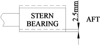
a) Parallel misalignment

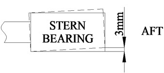
b) Angular misalignment

Vibration data was collected using accelerometers, which were attached with rubber bases to the ends of stern bearing as showed in the Fig. 9. Accelerometers were placed at the 9 o’clock position and 3 o’clock position at the front end and rear end of the stern bearing. One group (20480 points) was collected per minute with a sampling rate of 25.6 kHz. 160 groups of each condition were collected, and 80 groups are used for training the SVM model and another 80 groups were adopted for testing.

5. Results and discussion

In order to identify different working conditions of the monitoring bearing and stern bearing on propulsion shaft system, the proposed fault diagnosis method mentioned above is performed.

Fig. 10The CEEMD decomposition results of rolling bearing vibration signal with rolling element defects in 1750RPM

5.1. Case 1: fault diagnosis of bearing

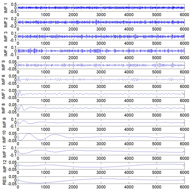
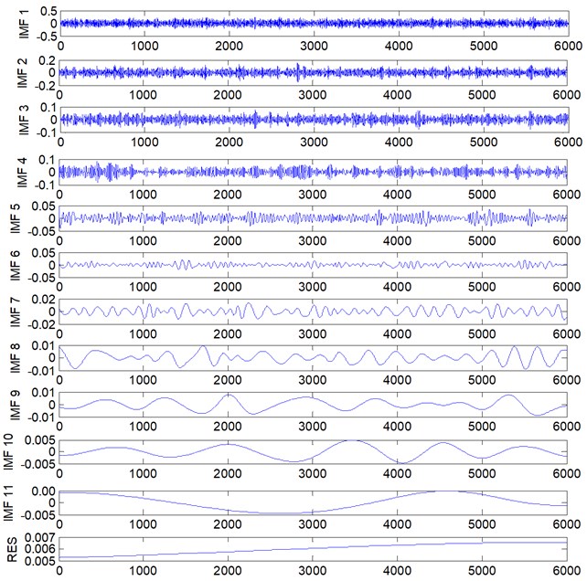
Firstly, the rolling bearing faulty signals are decomposed into several IMFs using PEEMD and CEEMD and the cost time are studied. The decomposition results of rolling element defects signal in 1750RPM through CEEMD and PEEMD are showed in Fig. 10 and Fig. 11, respectively. Since the IMFs of each signal are different and only the first IMFs contain the main faulty characteristic, the first five IMFs of each signal are selected. The statistical features, energy and kurtosis, of the five IMFs are calculated to construct a 10-dimensional feature vector. According to the faulty features classification method described in Section 3, the classification accuracies using all the PEEMD faulty features and using all the CEEMD faulty features are investigated. The results are listed in Table 2.

Table 2The feature extraction cost time (s) and fault diagnosis accuracies (%) of rolling bearing

Work load condition	Signal processing method	Cost time (s)	Classification accuracy
Condition 1 (1750RPM)	CEEMD	109.5	98.25 %
	PEEMD	27.0	99.25 %
Condition 2 (1797RPM)	CEEMD	105.9	98.50 %
	PEEMD	29.2	99.75 %

Fig. 11The PEEMD decomposition results of rolling bearing vibration signal with rolling element defects in 1750RPM

The results show that the calculating time of PEEMD save a great deal than CEEMD method. At the same time, the GA-optimized SVM recognition accuracies of using PEEMD faulty features are higher than using CEEMD faulty features. It indicates that the PEEMD method is more effective and need less calculating time than CEEMD method.

Meanwhile, considering the PEEMD faulty features, the recognition accuracies using all faulty features and using the extracted faulty features through PCA are researched. The results are listed in Table 3.

From Table 3, we can find that the recognition accuracies obtained using the selected faulty features through PCA are little more than those obtained using all faulty features.

Table 3The recognition accuracies (%) of rolling bearing obtained using all faulty features and using the selected faulty features through PCA

Work load condition	Classification accuracies using all features	Classification accuracies using selected features
Condition 1 (1750RPM)	99.25 %	99.50 %
Condition 2 (1797RPM)	99.75 %	100.00 %

6. Conclusions

In this paper, a novel fault diagnosis method based on PEEMD, PCA and SVM is presented. Firstly, the PEEMD method is employed for decomposing the vibration signal into IMF components. And the statistical features, energy and kurtosis, of the IMF components containing main faulty features are calculated for constructing the feature vector. Secondly, PCA is adopted for feature vector dimensions reduction. Finally, the GA-optimized SVM method is used for faulty condition recognition. The features extracted by this method had better distinction ability and cost less time, so it is more effective in faulty condition diagnosis. The validity of the proposed fault diagnosis method is verified by the application of practical experiments of the rolling bearing and stern bearing in the propulsion shaft system.