Abstract
Axially moving plates can be found in many industrial applications. Characteristics of the motion of thin moving plates are demonstrated in this paper using real-time signals and the Hilbert-Huang transform method. Ensemble empirical mode decomposition (EEMD) and calculation procedures are used to determine the instantaneous frequency, Hilbert spectrum and marginal spectrum of a moving plate. Some comparisons between different cases are discussed briefly. The motion is sensitive to the velocity, the initial tension of the conveyor strings and the weight of the plate. In addition, to express the motion (including the pitch and roll) of a moving plate quantitatively for field applications, a motion indicator is introduced. The signal processing method used is based on EEMD and time domain filtering. The indicator should be helpful for monitoring or adjusting the motions of axially moving plates.
1. Introduction
Axially moving continua can be found in many industrial applications, including conveyor belts, band saw blades, paper sheets, and magnetic tapes. The dynamics of axially moving systems have been studied for many years. Recently, a review of the characteristics of axially moving continua has been provided by Marynowski and Kapitaniak [1].
Compared with investigations of string-like and beam-like systems, the literature related to the dynamics of axially moving plates has not been extensive until recently. The earlier study of the vibration and stability of wide band saw blades was by Ulsoy and Mote [2], who discussed both approximate solutions based on the classical Ritz and finite element-Ritz methods and analytical results. Using linear plate theory and exact boundary conditions, the stability and vibration characteristics of two-dimensional axially moving plates has been investigated by Lin [3]. Because of the complexity of the mathematical model of an axially moving plate, many types of numerical methods have been used, including the mixed finite element method by Wang [4], the modal spectral element method by Kim [5], the finite strip method by Hatami [6, 7], the differential quadrature method by Zhou [8, 9], and the finite difference method by Yang [10]. Using the direct time integration method, Ghayesh and Amabili [11] explored the geometrical nonlinear dynamics of an axially moving plate. The time histories, bifurcation diagrams, Poincare maps, phase-plane portraits, and Poincare sections at points of interest in the parameter space were discussed. Ghayesh and co-workers [12] investigated the nonlinear dynamics of the forced motion of an axially moving plate numerically using the pseudo-arclength continuation technique and highlighted the effect of system parameters such as the axial speed and pretension on the resonant responses. With the help of an analytical approach, Banichuk [13, 14] investigated the limit velocity, buckling phenomena and the instability of axially moving membranes and plates. In addition, because industrial materials usually have viscoelastic characteristics, some researchers have taken an interest in viscoelastic moving panels, plates and webs [15-17].
There are only a few published experimental studies of axially moving continua. Through experimental and analytical methods, Moon and Wickert [18] investigated the nonlinear vibration of a power transmission belt system excited by pulleys and compared the theoretical and experimental results. Pellicano et al. [19, 20] experimentally investigated the instability and nonlinear resonances of a power transmission belt and presented comparisons between the analytical solution and experimental data. Xia et al. [21, 22] presented experimental results on the vibration characteristics of an axially moving string. Axially moving plates are members of a class of widely used engineering systems that has not yet been studied in depth experimentally. The present paper concentrates on the vibration characteristics of a poly-crystalline silicon solar wafer carried by a pair of parallel moving strings separated by a distance. Based on the experimental data, the time-frequency features of the moving wafer are analyzed using the Hilbert-Huang transform (HHT), which is considered a powerful time-frequency analysis method [23-25]. In Section 2, the experimental system and its parameters are briefly introduced. The transverse vibration features of the strings, the instantaneous frequencies, the Hilbert spectra and the marginal spectra of the moving plates (solar wafers in this case) are detailed using the HHT in Section 3. To monitor the motion through time-domain filtering and smooth the result using a regressive Gaussian filter, a motion indicator that describes the pitch and roll of the plate is presented in Section 4. Finally, some conclusions are stated in Section 5.
2. The experimental system
Fig. 1 shows a schematic of the test system, which includes two seamless parallel polyester strings that are 6 mm in diameter and separated by 90 mm. The parameters of the test system and the sample solar wafers are listed in Table 1.
Fig. 1A schematic of the test stands for measuring the vibrations of moving thin plates and the two strings
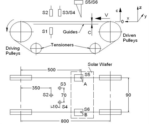
To drive the system, a step motor is used with different velocities. Two polytetrafluoroethylene guides that almost cover the span are arranged to reduce the string vibrations to an acceptable level. The clearance C (between the string and the guide) and the initial tension P in the strings can be adjusted separately. Two laser sensors of type ANR1251 are used for collecting the transverse vibration signals of the strings and the plate at positions A and B [21, 22]. Capacitance sensors S2 (of type Micro-epsilon capaNDCT6500 with a Ф10 mm probe) and S3 and S4 (of type DWS with Ф16.2 mm probes) are used to monitor the transverse vibrations of the thin plate. The capacitance sensor S1, coupled with S2, is for measuring the thickness of the plates, which is not covered in this paper.
In this experiment, the clearance C remains 1.4 mm and a set of uniform axial velocities, 152.5, 305, 457.5, 610, 762.5 and 915 mm/s, is used. Two initial tensions in the strings, 20.5 and 30 N, that correspond with different velocities are set by the tensioners (in the actual stand, four tensioners are used). The time series data for different cases are recorded by a computer through an A/D converter at a sampling rate of 8 kHz.
Table 1Parameters for the test system and the sample solar wafers
Variable | Value |
Diameter of the driving/driven pulley | 86 mm |
Length of the guide | 610 mm |
String mass per unit length | 0.0399 kg/m |
Eccentricities of the driving pulleys* | 25, 36 µm |
Eccentricities of the driven pulleys | 8, 25 µm |
Solar wafer size | 156×156 mm |
Weight of wafer #1 | 11.09 g |
Weight of wafer #2 | 11.08 g |
Weight of wafer #3 | 11.44 g |
*The driving and driven pulleys are paired up as follows: a driving pulley with an eccentricity of 25 µm matches a driven pulley with an eccentricity of 8 µm; in the other pair, 36 µm corresponds with 25 µm | |
3. The characteristics of axially moving plates
In this section, the vibration characteristics of moving plates are introduced based on the HHT. In the HHT method, one of two decomposition processes, empirical mode decomposition (EMD) and ensemble empirical mode decomposition (EEMD), can be selected according to the features of the signal and the goal of the signal processing. Through the HHT (including EEMD/EMD and time-frequency spectrum analysis), one residue and a finite number of intrinsic mode functions (IMFs), the instantaneous frequency (IF), the amplitude of each IMF, the time-frequency-energy distribution (Hilbert spectrum, HSP) and the marginal spectrum (MSP) can be obtained [23, 24]. Although it requires more computer time, EEMD has been chosen for this analysis to avoid possible inter-wave modulations and to suppress possible intermittences. The detailed calculation procedures are as described in [21, 22]. As for the moving plates, the vibrations of the strings shown in Fig. 1 are the excitation sources; the transverse vibrations of the parallel moving strings are briefly introduced in the following sections.
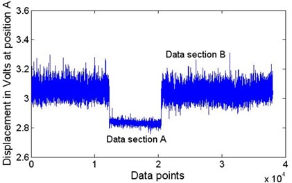
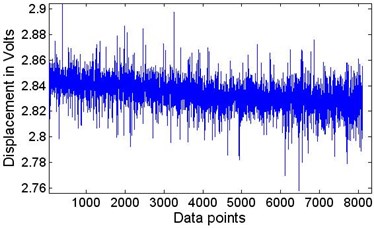
Fig. 2The original data measured by a laser sensor 5 when wafer #2 passed through position A at speed 152.5 mm/s. Data section A corresponds with the wafer’s transverse motion; Data section B corresponds with the string’s motion after the wafer has passed
3.1. Time-frequency vibration features of axially moving strings under load
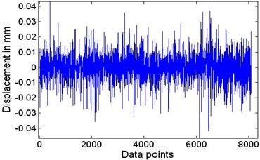
As shown in Fig. 1, there are two guides that constrain the vibration of each string unilaterally. The thin plate (in this experiment, only one solar wafer is carried by the strings at a time) is the load on the moving strings. Interactions between the strings, the guide and the plate influence the transverse motion of the strings. Two laser sensors, S5 and S6, collect real-time signals from positions A and B. Fig. 2 presents the original signal collected by S5. In this figure, data section A corresponds with wafer #2’s transverse motion, and data section B corresponds with the string’s motion after the wafer has passed. Taking a series of 15000 points from section B and decomposing it using EEMD, in which the ratio of the root-mean-square value of the added white noise to the standard deviation of the data series, , is set to 0.2, and the ensemble number is set to 400. Ten components and one residue (not shown here) are obtained. Fig. 3 shows the filtered signal in mm after the two highest frequency components and the residue are removed. The result of the significance test of the IMFs is presented in Fig. 4. The two highest frequency components are close enough to the white noise’s centre line that it is reasonable to cancel them out.
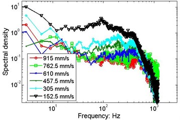
The MSPs for two speeds are shown in Fig. 5(a) and 5(b). At the same speed and initial tension, the spectral densities of positions A and B are not the same. There is a tendency for spectral density to decrease as the speed of the axial motion increases.
Fig. 3The vibration of the string at position A: A series of 15000 points taken from data section B in Fig. 2 is decomposed by EEMD; after the highest two IMFs and the residue are removed, the signal is reconstructed using the other 8 IMFs
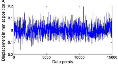
Fig. 4The results of the significance test of the IMFs corresponding with the series of 15000 points from data section B in Fig. 2
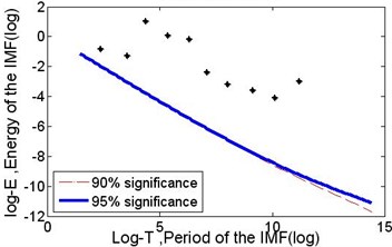
Fig. 5Marginal spectra of the string signals measured by S5 and S6 for wafer #2. The data series are from data section B
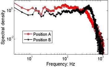
a) The MSP at a speed of 152.5 mm/s
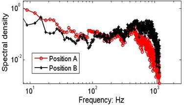
b) The MSP at a speed of 915 mm/s
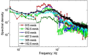
Fig. 6 presents the marginal spectra of the moving strings at different speeds. The variations in the MSP may be caused by discrepancies in the actual tension, clearance between the string and guide, eccentricity, or by the intrinsic non-stationary nonlinear characteristics of the vibrating strings.
3.2. Characteristics of the moving plates
In this experiment, the transverse vibrations of axially moving plates are observed at 6 speeds and two initial tensions in the strings. In addition to monitoring the motions of the strings, laser sensors S5 and S6, are used to collect the vibration signals of the plates. Capacitance sensors S2, S3 and S4 are only used for sensing the plates’ vibrations at different points. As an example, the analysis results at the lowest speed are presented below. In later sections, the results under different conditions are provided and some comparisons are made.
Fig. 6Comparisons of marginal spectra of the string signals measured by S5 and S6 under different speeds of axial motion. The data series are from data section B
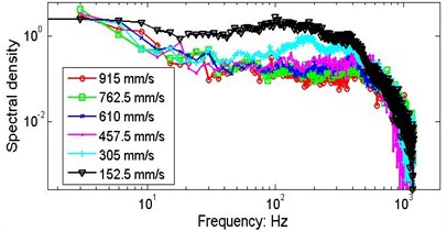
a) Position A, wafer #3, 20.5 N
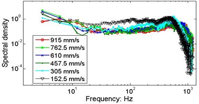
b) Position B, wafer #3, 20.5 N
c) Position A, wafer #2, 30 N
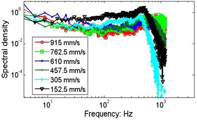
d) Position B, wafer #2, 30 N
3.2.1. Analysis of the moving plate’s signal at the lowest speed
Fig. 7(a) shows the original signal of wafer #2 moving at a speed of 152.5 mm/s measured by laser sensor S5 (corresponding with data section A in Fig. 2). Fig. 7(b) shows the filtered signal with the highest frequency component after the significance test [23] and the residue removed. EEMD ( 0.2, 400) is used to decompose the original signal and the results are shown in Fig. 8. Using the direct quadrature method [24] after the significance test against white noise is made, the instantaneous frequencies shown in Fig. 9(a) can be determined. In this picture, only the 9 frequency curves for IMFs 2-10 are presented; the highest-frequency component and the residue are left out. The corresponding centre frequencies are 537.9, 280.7, 151.2, 79.86, 40.6, 20.28, 11.32, 5.75 and 3.20 Hz. The time-frequency-energy distribution is shown in Fig. 9(b). Using calculation procedures [21, 23, 24], we can investigate the details of the plate’s vibration quantitatively.
Fig. 7The motion signal of wafer #2 moving at a speed of 152.5 mm/s
a) The original signal recorded by S5 at position A, 152.5 mm/s, 20.5 N
b) The filtered signal with IMF 1 and the lowest-frequency component of the residue removed
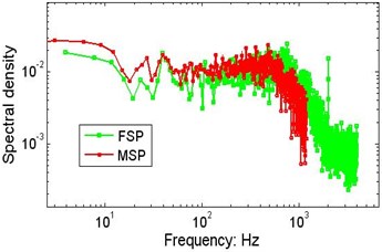
Fig. 10 shows the marginal spectrum and Fourier spectrum of the signal. Unlike the Fourier transform method, the HHT requires only a finite number of intrinsic mode functions (in this case the 9 IMFs obtained from the physical test signal) to express the original data series. The figure shows that there are two resonance peaks in the low frequency range.
Fig. 8The intrinsic mode functions of the signal shown in Fig. 7(a) as determined by EEMD, with the ratio of the root-mean-square value of the added white noise to the standard deviation of the data series σ= 0.2 and the ensemble number nt= 400; the residue is not shown
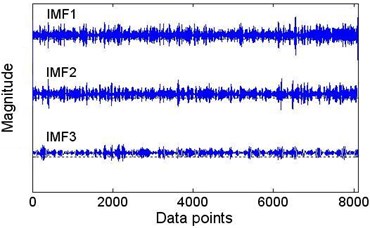
a) IMF 1, 2, 3
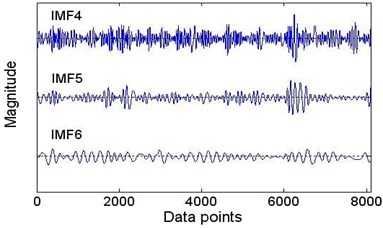
b) IMF 4, 5, 6
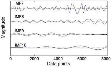
c) IMF 7, 8, 9 and 10
Fig. 9The instantaneous frequency and Hilbert spectrum of wafer #2 at a speed of 152.5 mm/s
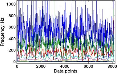
a) The IF calculated using the direct quadrature method, not including the highest component
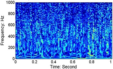
b) The HSP of position A
Fig. 10Comparison of the MSP and Fourier spectrum of wafer #2 at a speed of 152.5 mm/s and an initial string tension of 20.5 N
3.2.2. Comparisons of the behaviours of the moving plates under different conditions
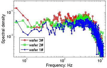
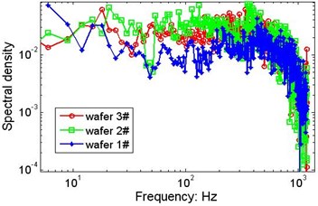
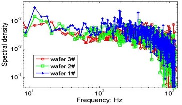
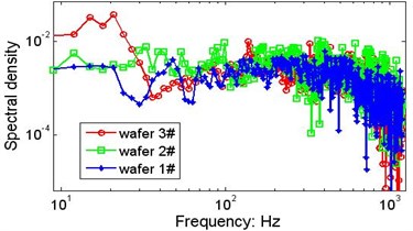
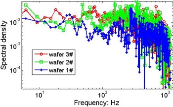
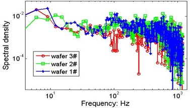
With the same system configuration, the vibration signals of the 3 wafers collected by laser sensors are analysed using calculation procedures similar to those mentioned above, and the marginal spectra are presented in Fig. 11. The weight difference between wafers #1 and #2 is very small, and the difference between wafers #2 and #3 is only 0.36 gram. Although the differences listed in Table 1 are relatively small, violent changes in the spectral density can be observed. In addition to the time-varying excitation from the strings, the slight difference in weight is one of the factors that may influence the vibrations of the plates, but it is difficult to determine the distinct contribution of the wafer’s weight.
Fig. 11Possible effects of the wafer’s weight on the marginal spectrum
a)152.5 mm/s, 205.6 N
b)305 mm/s, 205.6 N
c)457.5 mm/s, 205.6 N
d)610 mm/s, 205.6 N
e)762.5 mm/s, 205.6 N
f)915 mm/s, 205.6 N
Fig. 12The effect of the initial string tension on the marginal spectrum V= 152.5 mm/s
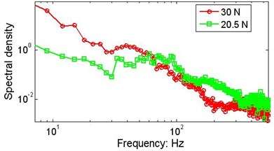
Fig. 12 shows the marginal spectra of wafer #2 measured by capacitance sensor S4 for different initial string tensions. For the larger values of the tension, the spectral density falls off more rapidly. Compared with the MSPs in Fig. 10 and 11, which are measured by laser sensors, the dominant frequency ranges of the MSPs measured by capacitance sensors in Fig. 12 and 13 are obviously within 100 Hz. This is probably caused by the averaging or aperture effect of the capacitance sensor. Fig. 13 shows marginal spectra for six speeds. In these figures, the marginal spectra vary dramatically because of the speed; in addition, there are resonant frequency areas that are approximately tens of Hz, but when the initial string tension is 30 N, the peak values are contained, as shown in Fig. 13(b).
Fig. 13The effect of the initial string tensions on the marginal spectrum at different speeds
a)20.5 N
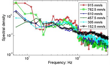
b)30 N
Fig. 14Low-frequency resonances at different speeds
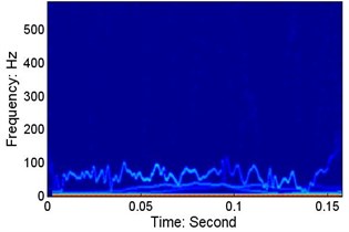
a)152.5 mm/s, 20.5 N, wafer #3
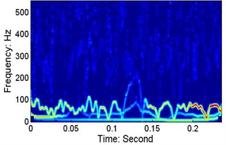
b)610 mm/s, 20.5 N, wafer #3
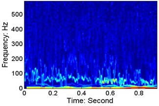
c)915 mm/s, 20.5 N, wafer #3
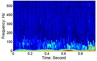
d)152.5 mm/s, 30 N, wafer #2
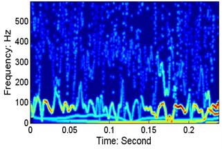
e)610 mm/s, 30 N, wafer #2
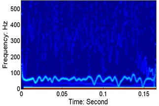
f)915 mm/s, 30 N, wafer #2
Fig. 14 presents the Hilbert spectra for six cases. At different speeds, there are low-frequency resonances in the wafer’s motion, and the centre frequencies (the mean value of the IF of the dominant IMF in each case, where the IF is obtained using the quadrature method) are: a) 58.16 Hz, b) 71.43 Hz, c) 63.83 Hz, d) 77.75 Hz, e) 73.28 Hz, and f) 60.79 Hz. As shown in Figs. 13 and 14, the lower resonance frequency area is not obvious when the capacitance sensor signals are used.
4. A motion indicator for the moving plate
A quantitative expression for the motion of a moving plate is of interest for engineering applications. Using real-time signals, we can define a motion indicator to characterize the plate’s pitch and roll. As shown in Fig. 15(a), P2, P3 and P4 correspond with sensors S2, S3 and S4, respectively. In the configuration of sensors shown in Fig. 1, the coordinates can be denoted as P2(0, 0, ), P3(10, 35, ) and P4(10, –35, ), in which , and are the transverse motions at points P2, P3 and P4. The motion vectors can be defined as:
in which the range of (the number of data points involved in the calculations) takes on different values for different speeds.
The motion indicator shown in Fig. 15(b) can be defined by:
That is the cross product of the two motion vectors.
To determine the -direction data series, first, the signals recorded by S2, S3 and S4 are decomposed using EEMD ( 0.2, 400). Then, an orthogonality check and a significance test are used to filter out the highest frequency components and the residue in the time domain, and the reconstructed data series can be obtained by combining the rest of the IMFs. The reconstructed data can be smoothed using a zero-order regression Gaussian filter with a cut-off frequency of 100 Hz [26]. Fig. 16 shows the smoothed displacement signal for a speed of 152.5 mm/s. As an example, for a speed of 152.5 mm/s, the transverse motion can be taken as (1:5775), (526, 6300) and (526:6300). Note that the three data series corresponding with these three points should be on the plate simultaneously. The maximum defined in Fig. 15(b) for speed 152.5 mm/s is 0.105764 degrees, the pitch angle range (around the -axis) is from +0.10574 till –0.084011 degrees, and the roll angle range (around -axis) is from +0.014196 till 0.01977 degrees.
Fig. 15Calculating the motion indicator
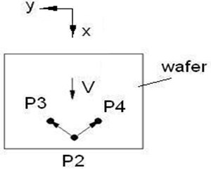
a) Motion vectors
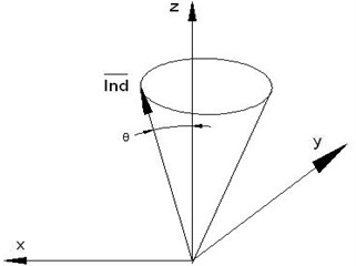
b) Indicator
Fig. 17 shows the motion indicators for wafer #2 at three different speeds. Among these variations, the pitch and roll angle ranges for a speed of 457.5 mm/s are from +0.0766 till –0.0812 and from +0.01182 till –0.01013 degrees; and for a speed of 915 mm/s, the ranges are from +0.5352 till –0.4515 and from +0.026296 till –0.02453 degrees, respectively. As shown in the figures, the tracks of the indicators vary with the speeds. The maximum strength of the pitching motion occurs when the speed is 915 mm/s. From an engineering application point of view, the indicator can present the motions of the plates intuitively.
Fig. 16The smoothed signal used to calculate the indicator, P= 20.5
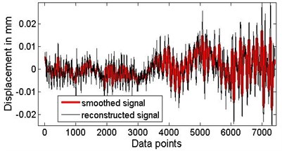
Fig. 17Motion indicators for wafer #2 with initial string tension 20.5 N
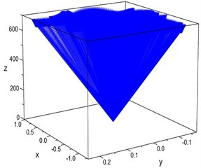
a) 152.5 mm/s
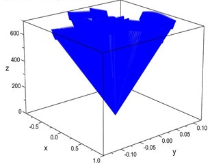
b) 457.5 mm/s
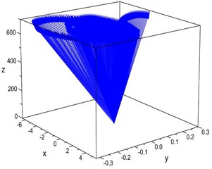
c) 915 mm/s
5. Conclusions
Moving plate systems often occur in engineering fields. Because of the complex interactions among the plate, strings and constraints in the system, mathematical modelling and analysis of the characteristics of moving plates in some physical systems are difficult to perform. Using real-time signals and a time-frequency method without any assumptions, we can obtain quantitative details of the motions of interest with physical significance, which is the key to actual applications.
In this paper, details of the motion of axially moving thin plates (solar wafers) are presented using the HHT method. The motions are sensitive to the moving speed, the initial string tension, and the weight of the plate. The vibrations different points on the plate are time-variant and should be nonlinear.
In addition, a motion indicator is introduced to quantitatively express the motion. Based on real-time signals and by time-domain filtering and frequency-domain smoothing, the indicator can be obtained in a straightforward manner. This should be helpful for monitoring the motions of plates used in some engineering applications, such as the measurement and sorting system for solar wafer quality control.
References
-
Marynowski K., Kapitaniak T. Dynamics of axially moving continua. International Journal of Mechanical Sciences, Vol. 81, 2014, p. 26-41.
-
Ulsoy A. G., Mote Jr. C. D. Vibration of wide band saw blades. Journal of Engineering for Industry, Vol. 104, 1982, p. 71-78.
-
Lin C. C. Stability and vibration characteristics of axially moving plates. International Journal of Solids Structures, Vol. 34, Issue 24, 1997, p. 3179-3190.
-
Wang X. D. Numerical analysis of moving orthotropic thin plates. Computers and Structures, Vol. 70, 1996, p. 467-486.
-
Kim J., Cho J., Lee U., Park S. Modal spectral element formulation for axially moving plates subjected to in-plane axial tension. Computers and Structures, Vol. 81, 2003, p. 2011-2020.
-
Hatami S., Azhari M., Saadatpour M. M. Free vibration of moving laminated composite plates. Composite Structures, Vol. 80, 2007, p. 609-620.
-
Hatami S., Ronagh H. R., Azhari M. Exact free vibration analysis of axially moving viscoelastic plates. Computers and Structures, Vol. 86, 2008, p. 1738-1746.
-
Zhou Y. F., Wang Z. M. Transverse vibration characteristics of axially moving viscoelastic plate. Applied Mathematics and Mechanics (English Edition), Vol. 28, Issue 2, 2007, p. 209-218.
-
Zhou Y. F., Wang Z. M. Vibration of axially moving viscoelastic plate with parabolically varying thickness. Journal of Sound and Vibration, Vol. 316, 2008, p. 198-210.
-
Yang X. D., Zhang W., Chen L. Q., Yao M. H. Dynamical analysis of axially moving plate by finite difference method. Nonlinear Dynamics, Vol. 67, 2012, p. 997-1006.
-
Ghayesh Mergen H., Amabili Marco Non-linear global dynamics of an axially moving plate. International Journal of Non-linear Mechanics, Vol. 57, 2013, p. 16-30.
-
Ghayesh Megen H., Amabili Marco, Paidousis Michael P. Nonlinear dynamics of axially moving plates. Journal of Sound and Vibration, Vol. 332, 2013, p. 391-406.
-
Banichuk N., Jeronen J., Kurki M., Neittaanmaki P., Saksa T., Tuovinen T. On the limit velocity and buckling phenomena of axially moving rothotropic membranes and plates. International Journal of Solids and Structures, Vol. 48, 2011, p. 2015-2025.
-
Banichuk N., Jeronen J., Neittaanmaki P., Tuovinen T. On the instability of an axially moving elastic plate. International Journal of Solids and Structures, Vol. 47, 2010, p. 91-99.
-
Saksa T., Banichuk N., Jeronen J., Kurki M., Tuovinen T. Dynamic analysis for axially moving viscoelastic panels. International Journal of Solids and Structures, Vol. 49, 2012, p. 3355-3366.
-
Tang Y. Q., Chen L. Q. Stability analysis and numerical confirmation in parametric resonance of axially moving viscoelastic plates with time-dependent speed. European Journal of Mechanics A/Solids, Vol. 37, 2013, p. 106-121.
-
Marynowski K., Kapitaniak T. Kelvin-Voigt versus Burgers internal damping in modeling of axially moving viscoelastic web. International Journal of Non-linear Mechanics, Vol. 37, 2002, p. 1147-1161.
-
Moon J., Wickert J. A. Nonlinear vibration of power transmission belts. Journal of Sound and Vibration, Vol. 200, Issue 4, 1997, p. 419-431.
-
Pellicano F., Fregolent A., Bertuzzi A., Vestroni F. Primary and parametric nonlinear resonances of a power transmission belt: experimental and theoretical analysis. Journal of Sound and Vibration, Vol. 244, Issue 4, 2001, p. 669-684.
-
Pellicano F., Catellani G., Fregolent A. Parametric instability of belts: theory and experiments. Computers and Structures, Vol. 82, 2004, p. 81-91.
-
Xia C. L., Wu Y. F., Lu Q. Q. Transversal vibration analysis of an axially moving string with unilateral constraints using the HHT method. Mechanical Systems and Signal Processing, Vol. 39, 2013, p. 471-488.
-
Xia C. L., Wu Y. F., Lu Q. Q. Experimental study of the nonlinear characteristics of an axially moving string. Journal of Vibration and Control, 2014, p. 1-15.
-
Huang N. E., Shen Z., Long S. R., Wu M. C., Shih E. H., Zhang Q. The empirical mode decomposition method and the Hilbert spectrum for non-stationary time series analysis. Proceedings of the Royal Society of London, Vol. 454A, 1998, p. 903-995.
-
Wu Z. H., Huang N. E. Ensemble empirical mode decomposition: a noise-assisted data analysis method. Advances in Adaptive Data Analysis, Vol. 1, Issue 1, 2010, p. 1-41.
-
Feng Z. P., Liang M., Chu F. L. Recent advances in time-frequency analysis methods for machinery fault diagnosis: a review with application examples. Mechanical Systems and Signal Processing, Vol. 38, 2013, p. 165-205.
-
Muralikrishnan B., Raja J. Computational Surface and Roundness Metrology. Springer-Verlag London Limited, 2009.
About this article

