Detection and identification of mechanical faults by Kalman filtering in electric machines

1. Introduction

Predictive maintenance studies are important especially in critical processes to ensure safe, reliable, and economic operation. To perform predictive maintenance actions, fault features have to be known a priori. These features can be determined from the collected data which is sensitive to faults by applying statistical methods and signal processing methods.

Induction motors are the most widely used electric drives in industrial processes and their monitoring is important for avoiding unscheduled downtimes. According to the statistical studies on distribution of failure causes of induction motors, about 50 % of motor failures are mechanical in nature such as bearing fault, shaft unbalance, misalignment, soft foot [1-7]. In this study eccentricity and bearing faults are considered. Eccentricity is non-uniform air gap between rotor and stator of the motor. Bearing faults are introduced in artificial way by applying electrical, thermal and chemical aging techniques on the motor. The vibration data is collected from healthy and faulty cases of motor during performance tests [6, 7].

Since it is not easy to determine the fault indicators from noisy time domain signals, some signal processing techniques are needed. The Kalman filter has been successfully used in aerospace applications and it is integrated into industrial systems. Kalman filter is a recursive state estimator and it is a good choice when there is modeling and measurement uncertainties. This filter can be also applied to non-stationary signals [8, 9].

Some of the studies related to signal based condition monitoring and fault diagnosis using Kalman filter can be given as follows: In [10], Kalman filtering applications to industry is overviewed. In [11], a review on filtering techniques in diagnostic studies is given. In [12], an extended Kalman filter is used to adjust the parameters of time-varying autoregressive model for gearbox condition monitoring. In [13], Kalman filter is integrated with support vector machine and applied to diagnose faults in rolling bearings. In [14], capability of Kalman filter using displacement signal for different noise sources in bearing fault identification is investigated. In [15], Kalman filter is integrated with recurrence quantification analysis to evaluate bearing degradation.

This paper consists of a case study about diagnosis of eccentricity and bearing faults in induction motor by Kalman filter based on autoregressive model of vibration signals and organized as follows. In Section 2 Kalman filter is given. In Section 3 eccentricity faults, ball bearing faults and experimental data is given. In Section 4 Kalman filtering application on vibration signals to detect mechanical faults is explained. In Section 5 the results are discussed, and the conclusions are given in Section 6.

2. Kalman filter

State estimation is the estimation of the state of a process with noisy measurements which is a common problem in science and engineering. Kalman filter which is introduced in the 1960s is the most widely used state estimator [8, 9]. It is a recursive filter and has been applied to linear or nonlinear dynamic systems. Some example applications are controlling the process in a chemical plant, predicting the flood in a river system, identifying the parameters in econometric models, tracking a spacecraft, navigating a ship etc.

Kalman filter is a recursive state estimator and consists of the prediction step using the process model and the correction step using the measurement model. The state-space equations of the system must be constructed to employ the Kalman filter. These equations can be obtained by signal based modeling method or physics based modeling method. In this study, Kalman filter will be constructed based on autoregressive model of the signals as explained below:

Let $s\left(k\right)$ be an autoregressive process of order $p$ that is generated according to the difference equation:

and suppose that $s\left(k\right)$ is measured in the presence of additive noise:

where $w\left(k\right)$ and $v\left(k\right)$ are the Gaussian white noise. The autoregressive model order $p$ can be determined by Akaike‘s information criteria and the autoregressive model coefficients $a_i$ can be determined by solving the Yule-Walker equations [8, 16-18]. Having found the autoregressive model, let $\underset{\_}{x}\left(k\right)$ be the $p$-dimensional state vector:

then Eq. (1) and Eq. (2) which is the formula for an autoregressive process can be arranged in state-space form as:

and:

These equations are simplified using matrix notation as:

where $A$ is a $p$ by $p$ state transition matrix:

is a vector noise process, $H$ is a unit vector of length $p$, and $T$ symbols transpose. Eq. (6) and Eq. (7) is called the state equation and the measurement equation respectively. Then the Kalman filter equations are given by.

Time update:

Kalman gain:

Measurement update:

where $\widehat{\underset{\_}{x}}\left(k|k-1\right)$ is the estimate of state vector $\underset{\_}{x}\left(k\right)$ based on the all measurement up to $k-$1. $w\left(k\right)$ and $v\left(k\right)$ are white noise processes with zero mean and covariance $Q$ and $R$. The parameters $Q$ and $R$ are related to modeling error and measurement error respectively, and the filter is sensitive to these parameters. $P$ is covariance of the estimation error of $x$. $K$ is the Kalman gain vector.

The innovation or residual sequence is defined as:

If the filter is optimal $e\left(k\right)$ is white noise with zero mean. Before the Kalman filter computation starts initialization has to be made for initial state and covariance vector as below:

where $E\left\{·\right\}$ denotes the expectation operator.

3. Eccentricity faults, ball bearing faults, and experimental data

Mechanical faults such as eccentricity and bearing faults are seen commonly in rotating machineries. Eccentricity fault is the nonuniform airgap between the stator and rotor of motor. This may occur due to misalignment of the shaft and damaged bearing. If the position of minimum airgap is fixed in space it is called static eccentricity, otherwise it is called dynamic eccentricity [2-5]. This type of fault can be recognized from the frequency spectrum of vibration signal located at the frequency components $f_r$, 2$f_r$, 2$f_e$, 2$f_e\pm f_r$, and 2($f_e\pm f_r$) where $f_r$ is the shaft frequency and $f_e$ is the supply frequency.

Bearing faults are caused due to wear, improper installation, improper lubrication, shaft currents, and manufacturing faults in the bearing components. Ball bearing faults are identified from the related frequencies of the bearing components. The four components of a ball (or rolling element) bearing are the inner race, the outer race, the rolling elements, and the cage. When there is a fault on these components vibration amplitude at related frequencies or their harmonics will increase. These frequency components are calculated using the bearing geometry as given in Appendix A1. However, when the bearing has rolling elements between 6 to 12 balls, approximate formulas given as follows can be used [7, 19]: Ball pass frequency of the inner race is $f_i=$ 0.6$N_b{f}_r$, ball pass frequency of the outer race is $f_o=$ 0.4$N_b{f}_r$, where $N_b$ is the number of balls, the cage frequency $f_c=$ 0.4$f_r$, and the ball spin frequency is determined using the bearing catalogue.

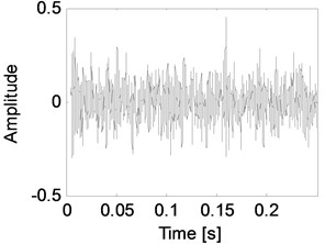
In this study, vibration data collected from healthy and faulty induction motor with damaged bearings are used. Bearing damage is artificially introduced by applying current to the motor shaft which causes to pass discharge currents at random on the surface of bearing components. Beside this type of damage called as fluting, the motor is subjected to thermal and chemical effects artificially to accelerate the aging [6, 7]. Vibration data is collected from healthy and faulty case of induction motor at 12 kHz sampling frequency and under full load condition by loading the motor with a dynamometer. An accelerometer is used to collect vibration data and it is located at 2 o’clock position of the drive-end side of motor.

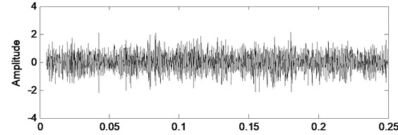
Fig. 1Healthy case vibration signal and its filtered version by Kalman filter

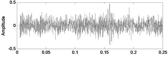
a) Original signal

b) Filtered signal

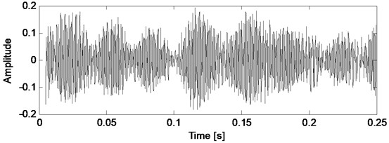
Fig. 2Faulty case vibration signal and its filtered version by Kalman filter

a) Original signal

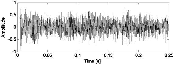
b) Filtered signal

4. Kalman filtering application on vibration signals to detect mechanical faults

In this study detection of eccentricity and bearing fault is considered. A state space model is needed to construct the Kalman filter, and it is obtained by autoregressive model of vibration data with sixtieth order determined by Akaike’s information criteria [16]. The parameters of Kalman filter which are modeling error and measurement error denoted as $Q$ and $R$ respectively, are selected as $Q=$ 10^-9 and $R=$ 10^-6 by trial and error. The vibration data acquired from healthy and faulty cases of motor and their filtered versions by Kalman filter are shown in time domain as seen in Fig. 1 and Fig. 2.

Fig. 3Power spectral density variations of healthy case vibration signal, filtered signal, and innovation

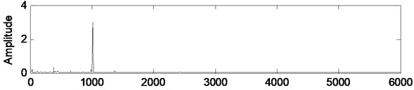
a) Original signal

b) Filtered signal

c) Innovation

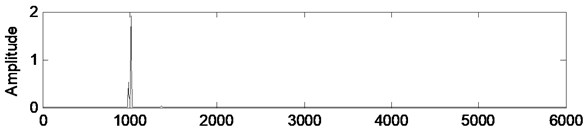
Fig. 4Power spectral density variations of faulty case vibration signal, filtered signal, and innovation

a) Original signal

b) Filtered signal

c) Innovation

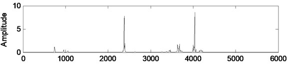
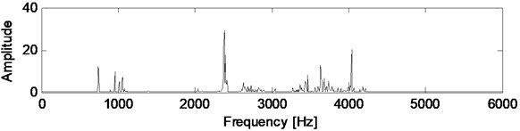
The motor is supplied with line frequency $f_e=$ 60 Hz. Rotor speed is 1742 cycles per minute, its corresponding rotating frequency is $f_r=$ 29.03 Hz. The number of balls in the bearing is $N_b=$ 9 and the characteristic bearing frequencies are calculated as $f_i=$ 156.7 Hz, $f_o=$ 104.5 Hz, $f_c=$ 11.6 Hz, and $f_b=$ 136.9 Hz. The eccentricity frequencies are 29.03 Hz, 58.06 Hz, 61.94 Hz, 90.97 Hz, 120 Hz, 149.03 Hz, and 178.06 Hz.

Fig. 3 and Fig. 4 presents the power spectral densities of original signal, filtered signal, and innovation or residual calculated as the difference between original signal and filtered signal for healthy and faulty cases. Computation of power spectral density is given in Appendix A2.

It is seen from Fig. 3(b) and Fig. 4(b) that the Kalman filter reduce the noise level and reduce the search space related to specific fault frequencies. In Fig. 4(b) the most dominant frequencies are identified as 744 Hz, 955 Hz, 2379 Hz, 2396 Hz and 3633 Hz. These frequencies correspond to following harmonics of fault frequencies taking into account that the frequency resolution is 5.85 Hz: 744 Hz $\approx$ 12×61.94 Hz; 5×149.03 Hz, 955 Hz $\approx$ 8×120 Hz; 7×$f_b$, 2379 Hz $\approx$41×58.06 Hz; 16×149.03 Hz, 2396 Hz $\approx$ 20×120 Hz, 3633 Hz $\approx$ 40×90.97 Hz.

Since there is an anti-aliasing filter with cutoff frequency at 4 kHz in the data acquisition system, the frequency components beyond that is not taken into account.

5. General discussions

5.1. Discussions on statistical analysis and spectral interpretations by Kalman filtering

In the field of rotating machinery condition monitoring and fault diagnosis, analysis of vibration signals is a common method since these signals can reflect many faults inside the machine such as unbalance, misalignment, eccentricity, bearing faults, soft foot, oil whirl. However these signals are complex due to their noise content. Extraction of fault features from these signals needs to apply signal analysis techniques. For this purpose, frequency domain methods, time-frequency/scale domain methods, stochastic methods, and soft computing methods are employed [20]. However, as a stochastic method, the Kalman filter applications on vibration signals in fault detection and diagnosis studies are in limited number in the related literature. In this study, the Kalman filter is considered to estimate vibration time series and to show its capability in fault diagnosis of rotating machinery from vibration signals through a real case study.

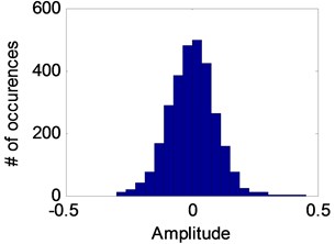
In order to make statistical comparison about the results of Kalman filter, the innovation signal or residual, which is the error between the original signal and its estimation obtained by Kalman filter, for healthy and faulty cases and their histograms are shown in Fig. 5. Also, time domain statistics of the original signal, filtered signal, and innovation signal are given in Table 1 for healthy and faulty cases.

Table 1Time domain statistics of the original signal, filtered signal, and innovation signal for healthy and faulty cases

	Original signals		Filtered signals		Innovation signals
	Healthy	Faulty	Healthy	Faulty	Healthy	Faulty
Mean	0.0016	0.0116	0.0004	–0.0008	0.0011	0.0123
Standard deviation	0.1102	0.6327	0.0715	0.2524	0.0917	0.6895
Skewness	0.0478	–0.0748	0.0205	–0.0179	0.0403	–0.0758
Kurtosis	3.0138	2.9882	2.3421	2.8373	3.5871	3.0053

From the Table 1, the most notable statistical parameter is standard deviation. Its value is reduced in healthy case of the original signal and innovation, but it increases in faulty case.

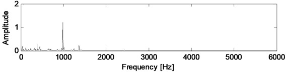
In Section 4, the specific fault frequencies are determined as 744 Hz, 955 Hz, 2379 Hz, 2396 Hz and 3633 Hz. Therefore, the interval of [744 Hz-3633 Hz] can be accepted as the frequency band of the faulty case. Hence this frequency band can be compared between original and innovation signals at the spectral domain as shown in Fig. 6. The symbol asterisk (*) used in Fig. 6(a) denotes a threshold value, and it is selected as 5.8 which is 20 % of the maximum amplitude. Here the numerical value of the threshold is considered to eliminate the undefined frequencies at 2631 Hz and 3439 Hz. On the other hand, the symbol circle (o) used in Fig. 6(a) denotes a threshold value for the frequency axis, and it is selected as the cutoff frequency of the filter (at 4 kHz) in data acquisition system. As seen in Fig. 6(a), there are two more frequency components which are 2631 Hz and 3439 Hz which are not harmonics of any specific fault frequencies. More simplified figure is shown as in Fig. 6(b) defined between threshold and lowpass filter limit used in Fig. 6(a).

Fig. 5a) The innovation signal for healthy case and b) its histogram, and c) the innovation signal for faulty case and d) its histogram

a)

b)

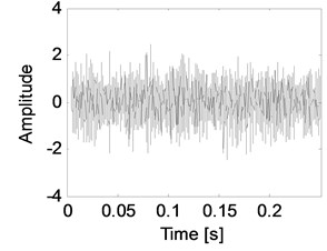
c)

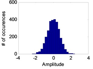
d)

Fig. 6a) Power spectral density variations of original signal and innovation signal for faulty case, and b) its simplified view

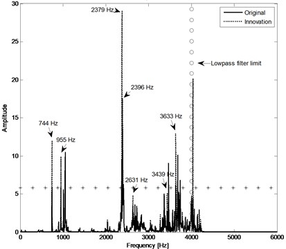
a)

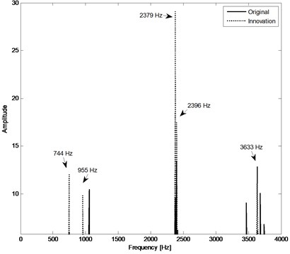
b)

6. Conclusions

Fault detection and diagnostic studies are important to prevent probable failures in advance. A number of signal based methods have been developed to extract fault features. This study is aimed to apply Kalman filtering to investigate its capability to detect the eccentricity and bearing fault using vibration signals collected from induction motors. State space model needed for Kalman filter is based on autoregressive models of vibration signals. Harmonics of the eccentricity and bearing fault related frequencies are identified using power spectral density variation of filtered vibration signal in faulty case. It is observed that Kalman filter reduce the noise level, and provide easy identification by decreasing the search space related to fault frequencies. And also, using the innovation signal of the Kalman filter, fault detection problems can be considered efficiently to detect the fault frequencies. However the filter is sensitive to process noise and measurement noise values. As a future work a systematic way of determining the optimal values of these parameters will be studied.