Abstract
Through curve fitting, the so-called flutter-margin method can estimate a good flutter boundary, however, is not suitable for the binary wing with a control surface. This paper develops the flutter-margin method and proposes a new stability criterion based on the dynamic equation of the three-dof wing and the Routh’s stability theory. The analysis of the trend and error-resistant ability show that: the new criterion, behaving a steady decrease to zero as instability is approached, varies in a sensibly linear manner with the velocity squared and could obtain good estimates of the flutter speed from data at a low speed, thus overcoming the defects of the velocity-damping method effectively. In addition, the criterion is more dependent upon the frequencies than on the decay rates, and is presented to be a good linear trend even when there is a 50 % damping maximum allowable error and 5 % frequency error.
1. Introduction
Flutter of aircraft is often a disastrous phenomenon, and thus it is essential to obtain the flutter boundary through wind tunnel and flight test [1]. But, considering the safety of life and property, it is difficult to reach the critical value of flutter. Traditionally, there is a flutter boundary prediction method so called velocity-damping method that fit and extrapolate the “trend” of the modal damping. When damping trend decreases to be zero, the airspeed is thought to be the flutter boundary [2-4]. Unfortunately, sometimes the modal aeroelastic damping of the nature flutter, especially so-called explosive flutter, will increase continually until just before instability, and then reduce suddenly. Furthermore, it is unknown which mode will go unstable, and certainly there will be some scatter in the modal damping measurements, thus lead to uncertainty about whether or not flutter will occur at the next increment of airspeed.
One method so-called “flutter-margin method” [5] is proposed to reduce this uncertainty. In this method, Zimmerman and Weissen burger make use of both the modal frequency and damping information and show that the flutter margin varies in a gradual manner with dynamic pressure. In particular when the instability is approached, the flutter-margin will decrease steadily to zero. Flutter experiments of a T-tail, a wing and a stabilizer have shown that the margin is applicable to two modes situation [5]. And more investigations of the use of the method have been done by Bennett [6] and Jennifer [7] on wind-tunnel aero elastic data and by Katz [8] and Lee [9] on flight test data.
However the margin can be used to binary instabilities only, then Price and Lee [10] developed a flutter margin method for three modes. Through the results of simulated experimental data, they proposed that the new margin will vary in a sensibly linear manner with dynamic pressure, thus could be a good tool to predict the flight flutter. But there is actually a mistake in their deducing process, and the simplified analysis of the margin is lack of rigorous.
In this paper, the flutter-margin method will be developed to the trinary flutter situation, and a new stability criterion will be proposed based on the dynamic equation of the three-dof wing and the Routh’s stability theory. The variation of this new criterion with airspeed will be described upon the simulated experimental data and the influence of modal parameter errors will be discussed latter.
2. The dynamic equation of the three-dof wing
Give a binary wing model with a control surface as shown in Fig. 1. The wing has three degrees of freedom: plunging motion , pitch motion and control surface yaw motion . The coordinate origin is set to be the center of the airfoil chord and the chord length is 2. In Fig. 1, , and represent the stiffness coefficient of each dof.
Fig. 1A binary wing model with a control surface
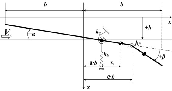
We can obtain the motion differential equation of the wing as follows:
where is aerodynamic force, is the aerodynamic moment for elastic axis, is the aerodynamic moment for hinge coordinate of the control surface.
Depend on Theodorsen’s theory [11], the quasi-steady aerodynamic force on the three-dof binary wing can be:
where - are configuration constants.
Substituting Eq. (2)-(4) into Eq. (1), we can obtain:
where -, - and - are configuration constants in derivation process.
Writing these equations in operational form with representing and performing some algebraic manipulations, they can be written as:
These three simultaneous differential equations in the unknown , and can be reduced to a single differential equation in each of the unknowns using straightforward operational techniques. If the unknown and are eliminated, we can get the differential equation for :
The exact expressions for the coefficients - are unimportant for our purpose, only the form or compositions are pertinent. The coefficients - take the form:
where the are configuration constants, our purpose is to gain the relationship between and airspeed , so it is unnecessary to know the expressions of .
From Eq. (11)-(12), since the depend on airspeed as well as on configuration, we also get that the resulting pitch motion will also vary with air speed. However, at any speed, Eq. (11) represents a linear differential equation whose solution is of the form:
where are the six roots of the corresponding characteristic equation:
The roots may be expressed in complex form as follows:
where is modal frequency and is modal damping. Substituting Eq. (15) into Eq. (14) and we have:
Then the Routh’s stability criterion is used to determine the stability boundary. This is done by forming the test determinants as follows:
The dynamic stability boundary is given by 0. And if is positive, we think the system is stable. At any speed, once the modal parameters and are measured, we can calculate the by Eqs. (16), (17). In order to be convenient to polynomial fit, we construct parameters as follow:
where are the function of , so they are configuration constants as well. - have the same function with - that proposed by Price [10], but there is difference between and . The is:
The reason caused the difference is that Price lost a “” in his deducing process. We perfect the , and plus it with , i.e. in Eq. (18), then we obtain .
If is positive, we think the system is stable. And when reduced to zero, the flutter is happen. Unfortunately, we can see from Fig. 2 that the variation of test function, i.e. , and (all normalized with respect to their maximum value), with is not particularly convenient for extrapolating from a subcritical airspeed to the flutter boundary. Therefore, we made an attempt to obtain a new test function which varies in a more convenient manner, and tried several different possibilities. The shown in Fig. 2 is a “better” choice. It should be stressed that all the test functions predicted exactly the same flutter boundary.
Fig. 2Variation of the normalized test function
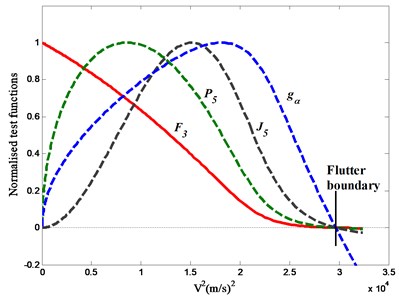
The test function for 3-dof wing is of the form:
Though is not a pure linear function of , as shown in Fig. 2, presents to be a convex function whose reduction rate decreases gradually when the airspeed approaching the flutter speed. We can use a linear fitting at low velocity to obtain a conservative prediction that is approximate to flutter. What’s more, because behaves a steady decrease to zero as instability’s approach, it will be helpful to overcome the defect of the velocity-damping method.
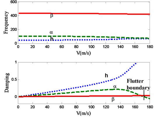
Fig. 3Modal parameters of the three motions at every velocity
3. Flutter boundary prediction
Construct a 3-dof wing with a control surface which have the follow structure parameters: 1.225 kg/m3, 0.3 m, 50.0 rad/s, 100.0 rad/s, 300.0 rad/s, 0.2, 0.0125, 0.25, 0.09, 40, –0.4, 0.6. The flutter was calculated through the - method, the flutter boundary is 172.2 m/s, and the graph of - and - is shown in Fig. 3.
Modal damping calculated by the - method can be approximated as the real decay rate of the vibration. So we can calculate at every velocity by the parameters in Fig. 3 through Eq. (16)-(18) and Eq. (20).
Depend on the model we also calculate the flutter margin in the Z-W method [5], which is of the form:
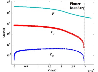
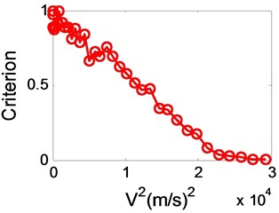
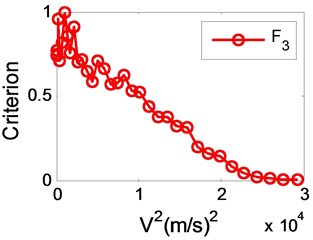
Then the was compared with the of Z-W method and the damping of the pitch motion, as shown in Fig. 4. When the velocity is approach to the flutter boundary, both the and the reduced gradually. However, while become to be zero at the flutter point, the is still positive. So the is not suit for the trinary flutter situation. In addition, although the damping decreased to zero as well when flutter is coming, the time its downtrend happened is so closed to the flutter speed that it is not useful to predict flutter boundary earlier.
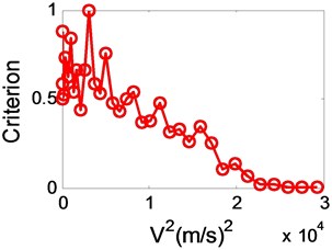
Fig. 4Variation of the criterions with velocity squared
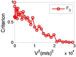
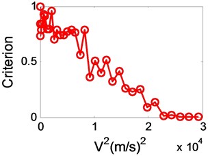
From Fig. 5(a) we can see that isn’t a pure linearity curve. It is nearly a linear function in the front part and present to be a convex function near the flutter boundary, as shown in Fig. 5(b). In the front part, the curve can be extrapolated to be a conservative prediction through linear fitting, and we call it the “first prediction”. will not decrease to zero at this point. After this velocity the curve belongs to the latter part that suit for linear fitting step by step with two or three points as the velocity increase.
Depending on linear fit, the predicted flutter boundary at every velocity is summarized in Table 1. At the front velocities, the predictions approach to 156 m/s and we define this speed to be the “first prediction”. Results of Table 1 show that: when airspeed is below than the “first prediction”, the prediction is toward to the “first prediction”; when airspeed is larger than the “first prediction”, the prediction is reaching true flutter boundary gradually. Though the “first prediction” is not equal to the true flutter boundary, in fact a little less than flutter, it is helpful for test personnel to get an approximate estimation and know how much the airspeed can be increased at a very low velocity.
Fig. 5Variation of F3 with velocity squared
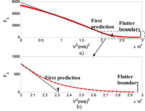
Table 1Predictions of the flutter speed at all the previous data points (true flutter is 172.2 m/s)
Before first prediction (m/s) | After first prediction (m/s) | ||||||
Current | Prediction | Current | Prediction | Current | Prediction | Current | Prediction |
34.0 | 181.7 | 102.0 | 165.3 | 150.0 | 155.0 | 167.0 | 170.1 |
51.0 | 177.8 | 119.0 | 160.7 | 155.0 | 160.6 | 170.0 | 171.5 |
68.0 | 173.8 | 136.0 | 156.5 | 160.0 | 164.6 | 171.0 | 172.0 |
85.0 | 167.7 | 153.0 | 156.2 | 164.0 | 167.8 | 172.0 | 172.2 |
4. Damping and frequency errors for 3-dof wing situation
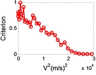
We have established that good predictions of the flutter speed can be obtained when accurate subcritical parameters are employed. However, because of the influence by noise, atmospheric turbulence, parameter identify method and other interferences, there are recognition errors in parameter identification progress inevitably. In order to decrease the recognition errors, Katz [8] used several sensors to measure modal parameters, and Copper [12] tried to reduce the interference of false modes. Koenig [13] gave exhaustive descriptions of the different sources of uncertainties encountered in flight vibration testing, and he noted that, even after a careful analysis of all available data, final scatter values of up to 2 % for frequencies and 35 % in damping were obtained on the good estimates. Ten years later [14], not much improvement was reported. For instance, a comparison of 16 different analysis methods is presented showing a scatter of approximately 3 % in frequency and 30 % in damping. For this reason, in order to see what is the effect on the flutter prediction of errors in the damping and frequency measurements, a maximum allowable error of 2 % and 5 % in frequency and 20 %, 30 %, 40 %, 50 % in damping were added in the previous case, the variation in with is shown in Fig. 6 and Fig. 7.
Though the variation in presented to have a scatter when there are large errors as shown in Fig. 6(d) and Fig. 7(d), it is convenient to use linear extrapolation to estimate the flutter boundary. On the other hand, comparing Fig. 6(b) with Fig. 6(a), error in damping increased from 20 % to 30 % when error in frequency is 2 %, it is apparent that the error in damping has produced very little deterioration in the variation in . Likewise, comparing Fig. 7(a) with Fig. 6(a), error in frequency changed from 2 % to 5 % as error in damping is 20 % all long, it shows that the effect of the error is to produce a fairly large scatter in . Because the recognition accuracy of modal frequency is much higher than that of damping, thus this law of errors effect to will help to predict flutter boundary accurately.
Fig. 6The trend graph of the criterion with 2 % frequency error and the following damping errors
a) 20 %
b) 30 %
c) 40 %
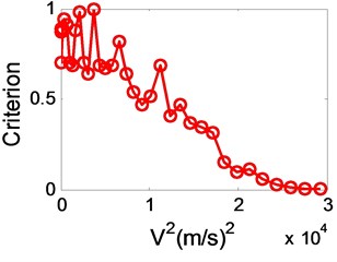
d) 50 %
Fig. 7The trend graph of the criterion with 5 % frequency error and the following damping errors
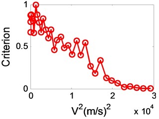
a) 20 %
b) 30 %
c) 40 %
d) 50 %
A summary of the effect of the errors is presented in Table 2. Generally, as errors of modal parameters increases, especially error in frequency, the accuracy of the estimated flutter speed decreases. When actual speed is low, like 85 m/s (50 % of the flutter speed) in the case A, we can obtain a flutter prediction. Though this prediction is not equal to the true flutter, it provides us the approximate range of the flutter. As the airspeed increased, like 100 m/s (60 % of the flutter speed) in the case B and 120 m/s (70 % of the flutter speed) in the case C, the predictions is closed to the “first prediction” (156 m/s, shown in Fig. 5) gradually. Meanwhile, when airspeed is larger than the “first prediction”, will decrease to zero as the speed approach to the true flutter. Unfortunately, no matter whether the airspeed is 85 m/s, 100 m/s or 120 m/s, the damping of the three modes in this example have no symptom to reduce, thus will have no help to predict flutter boundary in the velocity-damping method.
Table 2Effect of errors in frequency and damping measurements on the flutter predictions at the previous speed: A) 85 m/s, B) 100 m/s, C) 120 m/s – the true flutter is 172.2 m/s
Error | Prediction (m/s) | |||
Frequency, % | Damping, % | A | B | C |
2 | 20 | 154.9 | 167.5 | 162.3 |
30 | 151.8 | 159.9 | 156.5 | |
40 | 174.1 | 165.9 | 162.0 | |
50 | 210.4 | 163.9 | 169.5 | |
5 | 20 | 140.9 | 147.9 | 162.5 |
30 | 171.6 | 167.1 | 152.7 | |
40 | 215.9 | 166.9 | 156.3 | |
50 | 193.6 | 169.9 | 163.3 | |
5. Conclusions
A new stability criterion was proposed based on the dynamic equation of the three-dof wing and the Routh’s stability theory in this paper, and its variation with airspeed was described upon simulated experimental data. Further more, the influence of modal parameter errors was discussed through different combinations of maximum allowable errors. The results show that: 1) The criterion can help to predict an approximate flutter boundary with linear fit at low airspeed that will improve the security of flutter test. 2) There is a “first prediction” in the extrapolation process, and the significance of the “first prediction” is that, if airspeed is below than it, the prediction is toward to the “first prediction”, and when airspeed is larger than it, the prediction is reaching true flutter boundary gradually. 3) is shown to be relatively insensitive to errors in modal damping estimations, but is very sensitive to errors in modal frequency measurements. 4) Even in the worst situation, 5 % error in frequency and 50 % error in damping, good estimates of the flutter speed can be obtained from data at speeds as low as 60 % of the flutter speed.
References
-
Dowell E. H., Clark R., Cox D., et al. A Modern Course in Aeroelasticity. Chapter 5. Kluwer Academic, , , 2005.
-
Kordes E. E. Flutter Testing Techniques. NASA SP-415, 1975.
-
Walker R., Gupta N. Real-Time Flutter Analysis. NASA CR-170412, 1984.
-
Park C. G., Friedmann P. P. New time-domain technique for flutter boundary identification. AIAA, Dynamics Specialists Conference, 1992.
-
Zimmerman N. H., Weissenburger J. T. Prediction of flutter onset speed based on flight testing at subcritical speeds. Journal of Aircraft, Vol. 1, Issue 4, 1964, p. 190-202.
-
Bennett R. M. Application of Zimmerman Flutter-Margin Criterion to a Wind-Tunnel Model. NASA TM 84545, 1982.
-
Jennifer H. Stochastic Characterization of Flutter Using Historical Wind Tunnel Data. 48th AIAA/ASME/ASCE/AHS/ASC Structures, Structural Dynamics, and Materials Conference, 2007-1769, 2007.
-
Katz H., Foppe F. G., Grossman D. T. F-15 Flight Flutter Test Program. Flutter Testing Techniques, NASA SP-415, 1975, p. 413-431.
-
Lee B. H. K., Ben-Neticha Z. Analysis of flight flutter test data. Canadian Aeronautics and Space Journal, Vol. 38, Issue 4, 2002, p. 156-163.
-
Price S. J., Lee B. H. K. Evaluation and extension of the flutter-margin method for flight flutter prediction. Journal of Aircraft, Vol. 30, Issue 3, 1993, p. 395-401.
-
Theodorsen T. General Theory of Aerodynamic Instability and the Mechanism of Flutter. NACA-496 80N15047, 1979.
-
Copper J. E. Parameter Estimation Methods for Flight Flutter Testing. Advanced Aeroservoelastic Testing and Data Analysis, AGARD-CP-566, Vol. 10, 1995, p. 1-12.
-
Koenig K. Problems of System Identification in Flight Vibration Testing. AGARD-R-720, 1984.
-
Koenig K. Pretension and Reality of Flutter-Relevant Tests. Advanced Aeroservoelastic Testing and Data Analysis, AGARD-CP-566, Vol. 17, 1995, p. 1-12.
About this article

This research is partially supported by the National Natural Science Foundation of China (Grant No. 11172128 and No. 51475228), the Specialized Research Fund for the Doctoral Program of Higher Education of China (Grant No. 20123218110001), the Research Fund of State Key Laboratory of Mechanics and Control of Mechanical Structures (Nanjing University of Aeronautics and Astronautics) (Grant No. 0515G01), the Jiangsu Graduate Training Innovation Project (CXZZ13_0146) and the Priority Academic Program Development of Jiangsu Higher Education Institutions.
