A feature extraction method based on LMD and MSE and its application for fault diagnosis of reciprocating compressor

1. Introduction

Reciprocating compressors are one of the most popular machinery used in petroleum and chemical production processes, and their operational safety has become the significant subject of the intensive investigation and research with the increasing demand for high performance, safety and lower maintenance costs of the machinery [1, 2]. Vibration based measurement and analysis technique has proven to be highly effective in health monitoring and fault diagnosis of machinery and equipment for the abundant operational state information embodied in vibration signal [3, 4], and some of those techniques have successfully detected faults in rotating machinery such as gearbox and bearing under certain conditions [5, 6]. However, the vibration signals of reciprocating compressor have characteristics of nonlinearity, nonstationarity and multi-component coupling due to the factors such as clearance, nonlinear stiffness of bearings and the unbalanced and time-varying forces of components, and those traditional techniques, such as the time-domain statistical indicators and Fourier transform, may fail to extract effective features from the vibration signals in the fault diagnosis procedures of reciprocating compressor [7].

LMD is a novel self-adaptive time–frequency analysis method proposed by Smith [8]. It can self-adaptively decompose a complicated multi-component signal into a set of PF components, each of which is the product of an envelope signal and a purely frequency-modulated signal. Therefore, LMD is a suitable approach to deal with nonstationary, nonlinear and multi-component coupled vibration signal of rotating and reciprocating machinery. Recently, some scholars have studied the fault signal feature extraction methods based on LMD. Wang et al. [9] presented a demodulation method based on LMD, and extracted features from the real vibration signals of a gas turbine system to identify its rub-impact fault successfully. Cheng and Yang [10] used LMD to diagnose bearing and gear faults and achieved good effects.

In recent research, entropy is widely used to measure the regularity or orderliness of time series, and hence different calculations of entropy, such as the approximate entropy [11], pattern spectrum entropy [12], energy entropy [13], and sample entropy [14], are defined to characterize the system dynamics and disorderliness that are related to machinery defects and malfunctions. However, these single scale entropy algorithms yielded contradictory results when applied to real-world datasets, in regard to this, Costa [15] proposed a MSE procedure to calculate sample entropy over a range of scales to represent the complexity of a time series. The MSE has been successfully applied to the fault diagnosis of different machineries in the past decades. Lin [16] presented a novel approach based on MSE to discover features of misaligned motors.

The original signal of mechanical system has strong stochastic properties, and is susceptible to the noise interference, so it is necessary to pretreat the original signal by LMD before the MSE calculation for an accurate feature extraction. Liu [17] has presented a fault feature extraction method based on LMD and MSE to diagnose roller bearing faults, while only the MSE of first PF component was chosen as fault feature for pattern recognition, and the other PF components was ignored. To use information of all PF components, that is, to choose the entropy values from MSE of all PF components, may be a more effective feature extraction method.

In this research, we are interested in the feature extraction method based on LMD and MSE and its application for reciprocating compressor at different oversized bearing clearance faults. In Section 2 we present the LMD method. In Section 3 we explain the MSE method. In Section 4 we describe the steps of feature extraction method based on LMD and MSE. Feature extraction process for different reciprocating compressor bearing clearance states is presented in Section 5. Finally, conclusion is outlined in Section 6.

2. LMD method

LMD method decomposes a complicated signal into a set of product functions, each of which is the product of an envelope signal and a purely frequency modulated signal. For any signal $x\left(t\right)$, it can be decomposed as follows:

1) The first step of the decomposition involves finding out all the local extrema $n_i$ and calculating the mean of two successive extrema $n_i$ and $n_{i+1}$. So the $i$th mean value $m_i$ is given by:

All mean values $m_i$ of two successive extrema are connected by straight lines. The local means are then smoothed using moving averaging to form a smoothly varying continuous local mean function $m_{11}\left(t\right)$.

2) The $i$th envelope estimate $a_i$ is given by:

The local envelope estimates are smoothed in the same way as the local means to derive the envelope function $a_{11}\left(t\right)$.

3) The local mean function $m_{11}\left(t\right)$ is subtracted from the original data $x\left(t\right)$:

$h_{11}\left(t\right)$ is then divided by $a_{11}\left(t\right)$:

The envelope $a_{12}\left(t\right)$ of $s_{11}\left(t\right)$ can then be calculated. If $a_{12}\left(t\right)\ne$ 1, the procedure needs to be repeated for $s_{11}\left(t\right)$. A local mean $m_{12}\left(t\right)$ is calculated for $s_{11}\left(t\right)$, subtracted from $s_{11}\left(t\right)$, and the resulting function amplitude demodulated using $a_{12}\left(t\right)$. This iteration process continues n times until a purely frequency modulated signal $s_{1n}\left(t\right)$ is obtained.

In practice, a variation $\delta$ can be determined in advance. If $1-\delta \le a_{1(n+1)}\left(t\right)\le 1+\delta$ and $-1\le s_{1n}\left(t\right)\le 1$, then iterative process would be stopped.

4) The corresponding envelope $a_1\left(t\right)$ is given by:

Multiplying envelope signal $a_1\left(t\right)$ by the purely frequency modulated signal $s_{1n}\left(t\right)$, the first product function $P{F}_1\left(t\right)$ of the original signal can be obtained:

5) Subtract the first PF component $P{F}_1\left(t\right)$ from the original signal $x\left(t\right)$ and we have a new signal $u_1\left(t\right)$, which becomes the new original signal and the whole of the above procedure is repeated $k$ times until $u_k$ becomes a monotonic function:

Thus, the original signal $x\left(t\right)$ was decomposed into $k$ PF components and a monotonic function $u_k$:

where $u_k$ is the residual term, $k$ is the number of the PF components.

3. Multiscale entropy

4. The feature extraction method based on LMD and MSE

LMD can self-adaptively decompose a complicated multi-component signal into a set of PF components, and the state features in the first several PFs are more highlighted than those in original signal. MSE is an effective means of analyzing the regularity of a time series from multiple scales, and give a more detailed description of state features. The combination of LMD and MSE method can give a more precise description of the regularity of highlighted PF components. The combination process is as follows: firstly the signal of state $k$ ($k=\text{1}$,..., $w$) is decomposed by LMD; secondly the first several highlighted PF components are selected, furthermore the MSE values of the choosed PF components are calculated; finally the eigenvectors matrix is obtained as:

where $T_k$ is the eigenvectors matrix of the $k$th fault state, $n$ is the number of PF components, $m$ is the number of scale factor, $t_{p\tau }$ is the MSE value corresponding to the $\tau$th scale factor of $p$th PF component.

To form the state features only using the MSE of the first PF component, that is $t_{1\tau }$ ($\tau =$1,..., $m$), may neglect the critical state information of other PF components. However, superfluous features with MSE of all PF components may interfere with the diagnosis of machine faults, and inevitably result in the inaccuracy of identification as well as the increase of computational efforts. Therefore, it is beneficial to select the high-priority features among the large number of features for fault diagnosis purpose before the feature classification process.

To choose the MSE values for all PF components at one scale factor, such as $t_{p1}$ ($p=$ 1,..., $n$), is another way to form the state features, and this can extract features more comprehensive from the information of all PF components. While for the eigenvectors matrixs of different fault states, the MSE values are inconsistent for all scale factors. Some are relatively close, others are significant different. In order to ensure a better recognition accuracy of state features, a standard should be established to evaluate the scale factor of which the MSE values has the best divisibility between different fault states.

The implementation of this feature extraction process still has two issues to be resolved. One is the selection of highlighted PF components from LMD decomposition results for one fault state and the determination of consistent PF components number for all fault states, and the other is the establishment of standard to evaluate the divisibility of eigenvectors between different states.

LMD can decompose the state signal into a series of PF components, but not all of them are rich in state information, and usually the first several PF components contain the major information. Therefore, it is necessary to select the highlighted PF components for the convenient calculation. Correlation analysis reflects the similarity between two signals, so the correlation coefficient between the orignal signal and each PF component can be used for the selection. After setting a reasonable threshold value of the correlation coefficient, the highlighted PF components of each fault state are selected. While the number of PF components for different fault states may be inconsistent. To solve this problem, the PF component numbers of all fault states are summed, and then the sum is diveded by the number of states. The rounding average value of this quotient is used as the consistent number of PF components for all fault states.

Geometric distance of samples between different classes is a common standard to evaluate divisibility. Euclidean distance has advantages of easy calculation and a simple high-dimensional feature space conversion, so it is an effective standard to evaluate the divisibility of eigenvectors between different states. The Euclidean distance is calculated only between two eigenvectors, and the bigger it is, the better divisibility between the two eigenvectors is. While for more eigenvectors, the Euclidean distance between any two of all eigenvectors are calculated, and then the average value of all Euclidean distances can be used to evaluate the divisibility of these eigenvectors. Therefore, the Average Euclidean Distance (AVD) is emplyed as a standard to find the scale factor of which the MSE values has the best divisibility between different fault states.

Fig. 1The flowchart of this feature extraction method

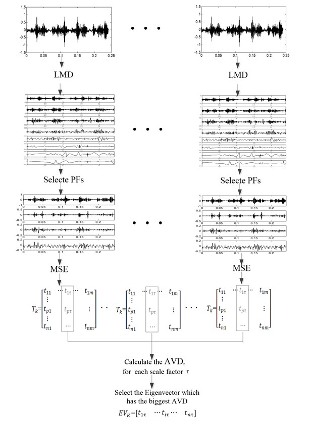
Based on the above discussion, the algorithm of this feature extraction method can be described as follow:

1) Decompose the vibration signals of different fault states into a series of PF components by LMD method;

2) Calculate the correlation coefficient between the orignal signal and each PF component, set a reasonable threshold value of correlation coefficient to select the first several PFs which contain major state information;

3) Sum the selected PF component numbers of all fault states, and divede the sum by the number of states $w$, then take the rounding average value of this quotient as the consistent number of PF components for all fault states;

4) Calculate the MSE values with a seris of scale factors for all selected PF components to form the eigenvectors matrix for all fault states;

5) Calculate the AVD between eigenvector $t_{p\tau }$ ($p=$ 1,..., $n$) of all fault states eigenvectors matrix $T_k$ ($k=$ 1,..., $w$) for each scale factor $\tau$;

6) Find the scale factor of which the MSE values has the best divisibility, that is, the bigger AVD, then take the eigenvector corresponding to this scale factor as the final eigenvector ${EV}_K=\left[\begin{array}{ccc}{t}_{1\tau }& \cdots t_{i\tau }\cdots & t_{n\tau }\end{array}\right]$.

The flowchart of this feature extraction method based on the above algorithm was shown as Fig. 1.

5. Fault diagnosis of reciprocating compressor

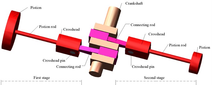
A two-stage double-acting reciprocating compressor of type 2D12, which is widely used to compress natural gas in chemical industry, was taken as the specific study object. The reciprocating compressor has a shaft power of 500 kW, a piston stroke of 240 mm and a motor speed of 496 rpm. The transmission mechanism of this compressor, as shown in Fig. 2, consists of crankshaft, connecting rod, crosshead, crosshead pin, piston rod and piston, and two ends of connecting rod are connected to crankshaft and crosshead pin by using sliding bearings respectively. Some clearances in its bearings are inevitable due to tolerances and defects arising from design and manufacturing process or wearing after a certain working period [18, 19]. The increased joint clearances can cause vibratory running condition which degrades compressor performances seriously.

Fig. 2A two-stage reciprocating compressor transmission mechanism

To study the diagnosis of bearing clearance states by vibration signal, four clearance fault states which include normal clearance state, slight worn, medium worn and severe worn of bearing between the crankshaft pin and first stage connecting rod was tested. This four clearance states are classified according to the four vibration grades of ISO 10816-6 standard. In the initial design and subsequent maintenance process, the clearance of this bearing is set as 0.05 mm to 0.1 mm, and the bearing in this clearance value is considered as normal clearance state. While based on several statistical results when the vibration monitoring of this bearing alarmed to avoid the damage of machine, the clearance value of this bearing is about 0.35 mm, and this clearance state is defined as severe worn clearance state. The 0.15 mm bearing clearance which corresponds to the acceptable for long-term operation is taken as slight worn state, and the 0.25 mm bearing clearance which is unsatisfactory for long-term continuous operation is defined as medium worn state in this test.

During the test a measurement point which is sensitive to the bearing clearance states was placed on the top of crosshead guide surface to collect vibration signal with an ICP acceleration sensor, as the triangle shown in Fig. 3, and the sample frequency is 50 kHz, the test of each state last for 4 s.

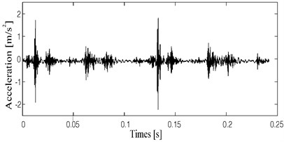
The typical vibration acceleration signals of the four bearing clearance states are shown in Figs. 4-7 for a period of two crank revolutions respectively. Compared to the chaotic vibration acceleration of normal state, the vibration acceleration of oversized clearance fault shows periodical shocks. The amplitude of shocks increases with the worn of bearing clearance gradually.

Fig. 3The structure of 2D12 reciprocating compressor

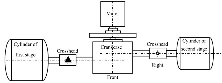
Fig. 4The vibration acceleration in normal bearing clearance state

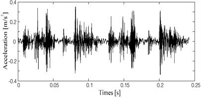
Fig. 5The vibration acceleration in slight worn bearing clearance state

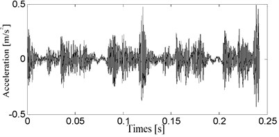
Fig. 6The vibration acceleration in medium worn bearing clearance state

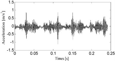
Fig. 7The vibration acceleration in severe worn bearing clearance state

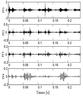
The vibration signals of four fault states were decomposed into a series of PF components by LMD, and then the correlation coefficient between the orignal signal and each PF component was calculated. Through the statistical analysis, the PFs components of which the correlation coefficient is larger than 0.1 contain the most state information. Therefore, by this threshold value of the correlation coefficient, the highlighted PFs components selected are 4 for normal clearance state, 4 for slight worn, 5 for medium worn and 4 for severe worn, respectively. Then the consistent number of PF components for all fault states is defined as 4. The first 4 PF components for all fault states are shown in Fig. 8 to Fig. 11.

The MSE values of the highlighted PFs components for four fault states were calculated. In this calculation process, the value range of scale factor $\tau$ was set as [1, 30], and the MSE values of each coarse grained time series $y^{\tau }$ were calculated with $m=$ 2 and $r=$ 0.15$\sigma$, where $\sigma$ denotes the standard deviation (SD) of the original signal. After the eigenvector matrixs of four bearing clearance states were obtained, the eigenvectors corresponding to the same scale factor was chosen from the four eigenvector matrixs respectively. Then the AVD between them was calculated, and this calculation process was conducted for all 30 scale factors.

To reflect the noise immunity of this method, 100 vibration signal samples are selected respectively from each bearing clearance states, and the MSE values of the highlighted PFs components were calculated. By compare the AVD between different scale factors, the best scale factor $\tau$ which has the biggest AVD is determined as 10. The average value and $\text{3}\delta$ (three times standard deviation) of eigenvectors corresponding to the best scale factor and its AVD were listed in Table 1.

Fig. 8The PF components of vibration acceleration in bearing clearance state

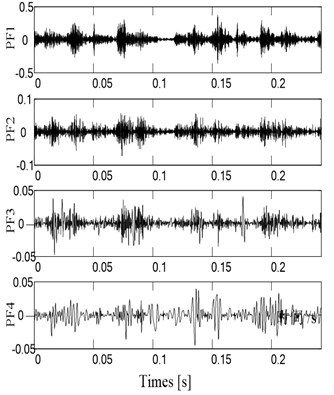
Fig. 9The PF components of vibration acceleration in slight worn state

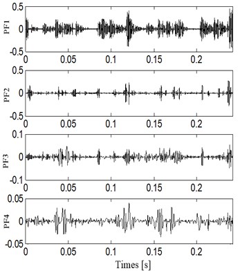
Fig. 10The PF components of vibration acceleration in normal state

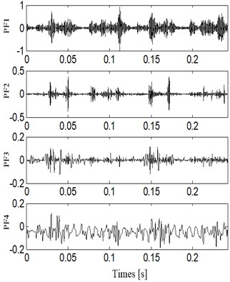
Fig. 11The PF components of vibration acceleration in slight worn state

In order to verify the superiority of this method, the sample entropy of the highlighted PFs components and their AVD were calculated for the above mentioned 100 vibration signal samples from each bearing clearance states, and the results were also shown in Table 1. We can observe not only the distribution of eigenvectors for MSE is wider than that of sample entropy, therefore the AVD is bigger, but also the $\text{3}\delta$ of eigenvectors for MSE is smaller than that for sample entropy.

In order to evaluate the effectiveness of feature extraction method based on LMD and MSE, Support Vector Machine (SVM) was used to recognize eigenvectors of four bearing clearance states. The toolbox LibSVM which was developed by professor Lin in Taiwan integrates parameter optimization, model training and test results, and it was used widely [20]. Kernel parameter and error penalty parameter $C$ are the main factors that affect the performance of SVM. In this article, the radial basis function is applied as kernel function, and its kernel parameter is $\gamma$. 100 eigenvector samples are selected respectively from each bearing clearance states, and 60 were used as training samples, other 40 were used as test samples. The kernel parameter $\gamma$ and error penalty parameter $C$ were optimized by genetic algorithm, and the optimization results is 1.94 for the error penalty parameter $C$, and 3.57 for the kernel parameter $\gamma$. The 40 test samples of each fault states were test by the trained SVM, and results are shown in Table 2.

To compare the effectiveness of this method, the same number of training and test samples were extracted by three other feature extraction methods which are LMD and sample entropy method, LMD and approximate entropy method, MSE method, and then three SVMs were trained and test by the same way. The recognition results are also listed in Table 2. We can kown that not only the accuracy of each state but also the total accuracy of the method used in this paper are higher than those of three other feature extraction methods. MSE calculates sample entropy over a range of scales, and gives a more detailed measure of complexity compare to sample entropy and approximate entropy; furthermore the proposed method has selection of scale factor, so it outperforms the combination for LMD with sample entropy and approximate entropy respectively. The state features in the first several PFs of LMD decomposition results are more highlighted than those in original signal, so the combination between LMD and MSE is superior to the single MSE method.

6. Conclusions

This paper presents a feature extraction method based on LMD and MSE, and it is applied for the fault diagnosis of reciprocating compressor at different bearing clearance states.

1) In the proposed method, LMD was used to decompose signal into a set of PF components, and the correlation coefficient was used to select the highlighted PF components which contain major state information.

2) The MSE values were calculated for all selected PF components, and the AVD was emplyed as a standard to find the scale factor of which the MSE values has the best divisibility between different fault states.

3) This method was applied for the fault diagnosis of reciprocating compressor at different bearing clearance states, and the effectiveness of this method is verfied by the recognition results of SVM compare to three other feature extraction methods.