Abstract
Complex diagnostic objects, e.g. critical rotating machines, usually generate a large number of diagnostic symptoms. A procedure is therefore required of selecting those most suitable from the point of view of technical condition evolution representation. A method based on the Singular Value Decomposition has been proposed for this purpose. An alternative is provided by an assessment of information content variation with time. Any symptom, treated as a random variable, may be assigned an information content measure that determines its ‘predictability’. As the end of service life is approached, symptom value is to a growing extent dominated by deterministic (and hence predictable) lifetime consumption processes, which implies decreasing information content. The symptom with the fastest decrease of an information content measure with time should thus be judged the most representative one. Suitability of such approach has already been demonstrated. The aim of this paper is to compare results obtained with both methods.
1. Introduction
The question of diagnostic symptoms selection was addressed at early stages of technical diagnostics development (see e.g. [1, 2]). Initially attention was focused mainly on malfunction detection and identification (qualitative diagnosis), so symptom sensitivity to condition parameters was the principal criterion. Further development brought about the question of damage extent determination (quantitative diagnosis) and then residual life assessment (prognosis) [3]. This implies a need to follow object condition evolution with time. The symptom which best represents this process should thus be considered the most suitable one.
Advanced diagnostic systems and procedures are obviously introduced for complex, costly and critical machines. Large power generating units provide a good example. Such objects typically generate a large number of diagnostic symptoms. Even if we limit our attention to vibration-based symptoms, this number still remains large and generally has no upper limit. Proper selection is thus of prime importance. Initially a method was suggested for this purpose, based on the Singular Value Decomposition (SVD) [4]. Suitability of this method for large steam turbines was studied by the author [5] and results were reported as satisfactory. The concept of employing Information Content Measure (hereinafter abbreviated to ICM) appeared later and initial results have been found promising [6]; further studies are under way.
ICM approach is based on the fundamental equation (see e.g. [7]):
where , , and indicate vectors of symptoms, condition parameters, control parameters and interference, respectively, and denotes time. If the influences of control and interference are neglected, any becomes a deterministic function of condition parameters. In a specific case, wherein elapsed time is the sole condition parameter, we arrive at the well-known symptom life curve, as given by the Energy Processor model [2]:
where is the initial power of residual processes, is the time to breakdown (both constant for a given object) and denotes symptom operator. Similar result is obtained when the vector is replaced by any scalar measure. It is easily seen that is a monotonically increasing smooth curve with the vertical asymptote given by .
In practice components of the and vectors can seldom be neglected. For a given object at a given location their components may be viewed random variables and it is reasonable to assume that they are described by time-independent statistical distributions. Observed time history is thus a superposition of two components, one deterministic and the other one random. While the latter does not change with time, the former is described by a relation of the type given by Eq. (2) and tends to infinity as . Symptom thus becomes more deterministic and hence more predictable, which is equivalent to information content decrease.
It may be argued that both SVD and ICM methods are based on the same underlying philosophy of information content assessment. However, whereas the former may be seen as employing information ʻdirectlyʼ contained in symptom time history, the latter concentrates on process organization around a monotonically increasing symptom life curve. It is therefore of interest to check if these different approaches lead to similar results. Application of both these methods was discussed by the author in an earlier publication [8]; however, no direct comparison of results has yet been attempted.
2. Symptom selection methods – an overview
2.1. SVD method
SVD approach is based on methods well known from linear algebra; detailed treatment can be found in specialized reviews and monographs (see e.g. [9]), while diagnostic applications have been dealt with elsewhere [4-6].
Let us assume that we have symptoms and readings of each symptom. This implies that, in principle, we are able to trace up to independent faults. The entire symptom database can be transformed into the symptom observation matrix . In order to make all symptoms comparable, irrespective of their physical origins, they are normalized with respect to their initial values and then 1 is subtracted, so that all become dimensionless and start from zero. By convention, elements of the singular values matrix :
where , are arranged in a descending order; in such case is uniquely determined by . The th generalized fault is characterized by the singular value and the sum:
can be interpreted as a measure of lifetime consumption and thus of overall object condition. SVD calculations allow for determining the contributions of condition parameters (ʻinputʼ) and measurable symptoms (ʻoutputʼ) into the singular value and hence into the th fault profile. Obviously the latter representation is the useful one, as condition parameters are typically nonmeasurable.
In practical applications [5, 8] it has been noted that for small values of no dominant singular value can be distinguished. This is interpreted as a mainfestation of the fact that no dominant failure mechanism has yet appeared. With increasing , however, this changes and typically a singular value with the highest contribution into the generalized fault (cf. Eq. (4)) can be identified. SVD analysis results point out the symptoms with the highest contributions into this singular value. This is the basis of the selection.
2.2. ICM method
As already mentioned, in practice any diagnostic symptom can be considered a random variable with time-dependent parameters. For a set of measurement data (equivalent to a column of the symptom observation matrix) a time window of constant width may be introduced, which is moved along the axis. Data points within this window are used to determine an experimental histogram, to which a statistical distribution is fitted. Weibull and gamma distributions have been found suitable, as they are compliant with more general requirements for diagnostic symptoms, such as 0 or long right-hand tail, as no upper limit value can usually be imposed on a symptom [6]. Parameters of these distributions will thus vary with time.
For any random variable we may speak in terms of information content and relevant measure. First such measure was introduced by Shannon in 1948 [10] and later termed Shannon entropy. It is given by:
where is a constant depending on the units used and denotes the probability of the th event. Logarithm base is typically 2, Euler’s constant or 10. Shannon entropy was originally introduced for verbal communication and is thus of discrete nature. For continuous random variables a measure known as continuous or differential entropy was formulated as (see e.g. [11]):
Despite formal similarity, continuous entropy is not the limit case of for . In particular, is non-negative, while may be negative (although the problem of negative information content still remains to be resolved). It can be shown, however, that for a given case time histories of Shannon and continuous entropies are just mutually shifted along the vertical axis. In view of what has been stated in Section 1, the shape of entropy versus time is of interest here rather than its absolute value. This implies that continuous entropy can be used for diagnostic symptom assessment, which simplifies calculations, as for commonly used statistical distributions this quantity is given by relatively simple analytical expressions, namely [12]:
for Weibull distribution, and:
for gamma distribution and:
for normal distribution; and denote shape and scale parameters, respectively, is the standard deviation, is the gamma function and is the Euler-Mascheroni constant. Normal distribution has been included here despite the fact that it is not compliant with all relevant requirements. The reason is that results obtained with this distribution have been found consistent with those obtained with Weibull and gamma distributions and qualitative conclusions have been virtually identical. Fig. 1 shows an example of fitting results, which illustrates this observation.
It may be added that several other information content measures have been proposed e.g. by Hartley [13], Rényi [14] or Tsallis [15]. However, either their suitability is limited to rather specific cases or there are fundamental problems with interpretation of certain parameters that appear in relevant formulas. Shannon entropy is still in common use.
Fig. 1Example of fitting results for normal (N), Weibull (W) and gamma (G) distributions
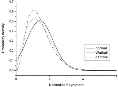
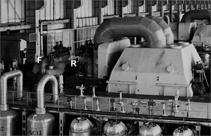
Fig. 2Photo of a 200 MW turbine unit. Locations of high-pressure turbine bearings is indicated by F (front bearing) and R (rear bearing)
3. Procedure and experimental validation
Symptom selection procedures shall be illustrated by experimental data obtained with the high-pressure turbine fluid-flow system of a 200 MW unit, operated in a utility power plant. This unit was commissioned in early 1970s and underwent modernization in 1994. Vibration measurements in the off-line mode were started shortly afterwards and continued until unit decommissioning in 2013. Available database covers over sixteen years and average period between consecutive measurements was about sixty days.
Although proposed symptom selection methods are applicable irrespective of symptom physical origin and method of acquisition, some information is provided for completeness:
– measured quantity: absolute vibration velocity;
– measurement points: front and rear high-pressure turbine bearings, in three mutually perpendicular directions;
– frequency range: 10 kHz;
– type of spectral analysis: 23 % constant percentage bandwidth (CPB);
– all symptoms are normalized with respect to their values at 0.
Fig. 2 shows the turbine unit and location of front (F) and rear (R) bearings. Measurements were performed using a Brüel & Kjær 4391 piezoelectric accelerometer and Brüel & Kjær 2526 MK2 data collector. Sentinel™ software package was used for general management of measurement results.
Frequency bands that contain components generated by high-pressure turbine fluid-flow system were determined from the vibrodiagnostic model (for details see e.g. [7, 8]). In this particular case, there are ten such bands that fall within so-called blade frequency range. With two measurement points and three directions, this gives sixty symptoms to choose from.
3.1. Measurement data pre-processing
Due to the influences of control and interference, symptom time histories in the blade frequency range are usually very irregular [16]. As already mentioned, their fluctuations reflect the random nature of diagnostic symptoms. However, certain values differ so much from the ‘average’ that they have to be qualified as outliers. It has to be stressed that while fluctuations as such are responsible for unpredictability and hence information content, outliers are, from the point of view of information theory, treated as noise and should be eliminated.
There is no precise definition of an outlier and no ‘universal’ method of removing them [17, 18]. The so-called ‘three-sigma rule’ employs a measure of ‘outlyingness’ in the form of [18]:
and assumes that if 3, then should be regarded an outlier. This rule is, however, not applicable for long-tailed distributions. The author has proposed a procedure referred to as ‘peak trimming’ [6], based on an assumption that if:
or:
then is treated as an ‘upper’ or ‘lower’ outlier, respectively, and replaced by:
Upper and lower threshold values should be adjusted experimentally. For vibration-based symptoms in the blade frequency range, 1.5 and 0.7 have been shown to give reasonable results.
In order to highlight another important issue related to measurement data pre-processing, we shall recall the time window procedure. In order to determine statistical parameters within such window, at least weak stationarity is required. While for small values of , where the increasing monotonic trend is still weak, this condition is (approximately) fulfilled, with approaching it is no longer the case. It is thus reasonable to speak in terms of fluctuations related to a trend rather than from some mean or average value [19]. In this particular case, the simplest solution is to introduce trend normalization, wherein symptom value is replaced by given by:
where lower index indicates value determined by the trend. is obtained by fitting continuous monotonic function to experimental data. Exponential fitting has been demonstrated to give good results, providing that is not too close to .
3.2. Entropy calculations
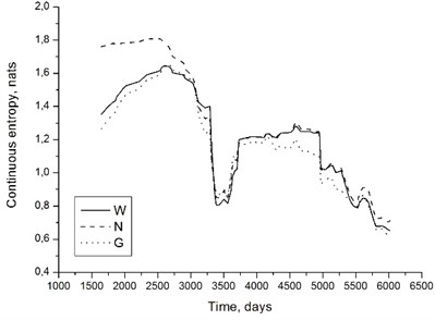
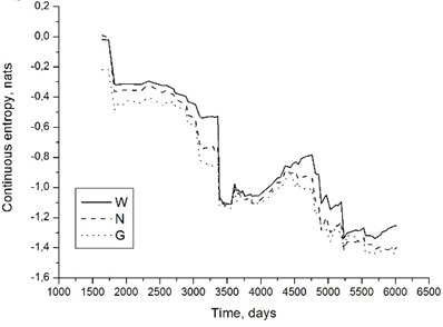
Fig. 1 suggest that evaluation results should be fairly insensitive to assumed symptom distribution type. This observation has been confirmed in practice. Fig. 3 shows examples of entropy time histories for the unit under consideration. Values of have been calculated from Eqs. (7)-(9).
It is easily seen that, despite some differences, all three distributions yield results that, from the qualitative point of view, are very similar. If we are reasoning in terms of entropy decrease with time, symptom assessment results shall not be affected by distribution choice. We may thus employ normal distribution, which is convenient from the point of view of calculations. Moreover, certain software packages sometimes reject data when fitting Weibull or gamma distribution, if the fitting algorithm is attempting to ‘stretch’ the probability distribution function onto the region of negative symptom values. Normal distribution does not have this disadvantage.
Fig. 3Continuous entropy time histories determined with the assumptions of Weibull (W), normal (N) and gamma (G) distributions; 200 MW unit, front high-pressure turbine bearing, horizontal direction, 5 kHz band a) and rear high-pressure turbine bearing, axial direction, 2 kHz band b). Entropy given in nats (b=e in Eq. (6))
a)
b)
3.3. Representativeness factor
A question may be asked if the rate of entropy drop with time (i.e. the value of ) should be accepted as the sole criterion of symptom suitability. From earlier considerations it may be stated, in a somewhat descriptive manner, that with increasing we observe the phenomenon of process organization about some monotonically increasing curve, namely symptom life curve. Entropy is a measure of this organization. In such approach, the symptom life curve is in fact neglected.
Fig. 4Normalized symptom (squares) and continuous entropy (circles): 200 MW turbine unit, front high-pressure turbine bearing, horizontal direction, 8 kHz band. Entropy given in nats (b=e in Eq. (6))
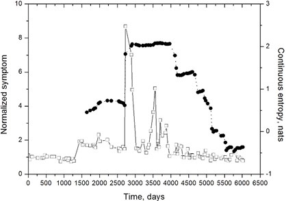
The problem is illustrated by an example shown in Fig. 4. It is easily seen that, apart from some apparently random fluctuations that have not been removed by peak trimming, symptom evolution is very slow and increasing trend almost unnoticeable. On the other hand, there is a strong entropy decrease starting about 4000 days, which indicates a high degree of process organization. We may conclude that this organization does take place, but about a curve that is fairly insensitive to object condition parameters, in this case represented by .
A measure should thus be conceived in the ICM method that would combine both entropy decrease and sensitivity to object condition. Such measure may be referred to as the representativeness factor . The simplest approach is to assume that the following approximations are valid:
and define . With such assumptions, should be positive and as high as possible; obviously positive values of resulting from negative and negative should be rejected. Approximations given by Eqs. (17) and (18) are quite rough – especially the latter – and suitable only for qualitative comparison. Such combination of two criterions seems, however, more meaningful than any of them alone.
4. Results and discussion
Although both methods can be employed irrespective of the number of symptoms, for the sake of clarity an initial selection has been performed. For each measurement point and direction, SVD method has been used to identify two most representative symptoms. An example is shown in Fig. 5. In this manner, twelve symptoms for further analysis are selected.
Fig. 5200 MW unit, front high-pressure turbine bearing, horizontal direction; a) contributions of individual singular values into the generalized fault; b) contributions of individual symptoms into three first singular values. Time elapsed θ has been accounted for as a symbol labelled 1, hence the number of symptoms is eleven
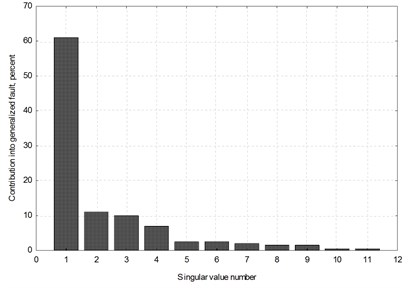
a)
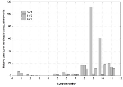
b)
Situation illustrated in Fig. 5 may be considered typical for a turbine with long operational record. In Fig. 5(a) it is clearly seen that one singular value is dominant, with the contribution into the generalized fault of over 60 percent. This means that dominant failure mechanism has already formed. Fig. 5(b) shows in turn that contributions of two symptoms – labelled 9 and 10 – into first three singular values are dominant, a few times higher than those of the remaining ones. These symptoms are selected for this particular measurement point and direction.
SVD analysis results are given in Fig. 6, in the form of contributions of individual symptoms into first three singular values (as in Fig. 5(b)). ICM analysis results, namely representativeness factor values for all twelve symptoms under consideration, are listed in Table 1. As normalized symptom is dimensionless and is equal to the Euler’s constant, these values are given in nats/day.
It is immediately seen that results obtained with two methods are not entirely consistent. SVD analysis obviously identifies symptoms 3 and 4 as the most representative ones; symptoms 1, 2 and 9 fare much worse and the remaining seven are of little significance. On the other hand, ICM analysis, while revealing comparatively high values of for symptoms 3 and 4, identifies symptom 5 as the best one and symptoms 6 and 10 as only slightly worse than 3 and 4; at the same time, symptoms 1 and 2 are completely rejected and symptom 9 is characterized by low value of .
Fig. 6Results of the SVD analysis for twelve symptoms pertaining to the fluid-flow system of the 200 MW unit high-pressure turbine
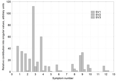
Table 1Results of the ICM analysis: representativeness factor values for twelve symptoms pertaining to the fluid-flow system of the 200 MW unit high-pressure turbine
Symptom number | Measurement point | Direction | Frequency band [Hz] | Representativeness factor [nat/day] |
1 | Front high-pressure turbine bearing | Vertical | 6300 | –0.63×10⁻⁸ |
2 | 8000 | –15.30×10⁻⁸ | ||
3 | Horizontal | 5000 | 6.97×10⁻⁸ | |
4 | 6300 | 5.57×10⁻⁸ | ||
5 | Axial | 6300 | 8.84×10⁻⁸ | |
6 | 8000 | 3.77×10⁻⁸ | ||
7 | Rear high-pressure turbine bearing | Vertical | 5000 | –1.93×10⁻⁸ |
8 | 8000 | 1.17×10⁻⁸ | ||
9 | Horizontal | 6300 | 0.20×10⁻⁸ | |
10 | 8000 | 4.14×10⁻⁸ | ||
11 | Axial | 2000 | –2.52×10⁻⁸ | |
12 | 8000 | 5.69×10⁻⁸ |
How can we comment on this observation? First, it is necessary to keep in mind that neither SVD nor ICM method can be considered the reference one. Both are based on certain assumptions. In view of that, we may argue that symptoms that are qualified highly representative by both these methods should be considered the most suitable ones for overall damage assessment. Such approach certainly minimizes the possibility of an erroneous classification. In this particular case, symptoms 3 and 4 are selected.
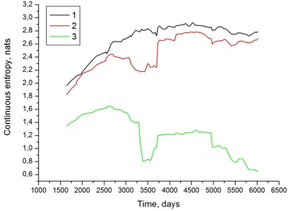
Second, it has to be kept in mind that both SVD and ICM results are to a certain extent influenced by data pre-processing, especially outlier removal method. A single outlier, if not removed, may significantly influence distribution fitting results. Peak trimming is a simple procedure which probably could be improved. Fig. 4 clearly shows that this method fails in certain cases, as some values that obviously ‘should’ be qualified as outliers have not been removed. ICM method is also sensitive to trend normalization. While the assumption of an exponential trend simplifies calculations, it is based on approximation which fails with . In first studies by the author (see e.g. [6, 8]) such assumption was shown to give good results. An example is shown in Fig. 7, which shows continuous entropy as a function of time for the symptom labelled 4 in Table 1. It is clearly seen that both raw and peak-trimmed data yield increasing entropy and only trend normalization reveals its decrease, which is consistent with theoretical results.
An improvement might probably be achieved by employing functions with a vertical asymptote, such as Weibull or Fréchet. Moreover, multiplicative normalization as in Eq. (14) is not supported by theoretical considerations. In fact, the Energy Processor model is additive, so additive normalization might be employed, with Eq. (14) replaced by:
On the other hand, transformation from the power of residual processes to measurable symptoms is nonlinear, irrespective of the symptom operator, which means that additivity is also not supported by the model. First attempts to employ Eq. (17) inevitably led to negative symptom values. It seems that this question requires further detailed analysis based on the Energy Processor model principles.
Fig. 7Continuous entropy vs. time for symptom labelled 4 in Table 1 and Fig. 6; 1 – raw data, 2 – peak-trimmed data (ch= 1.5, cl= 0.7), 3 – peak trimming with exponential trend normalization
It also has to be stressed that all above considerations are based on the assumption that we are dealing with a single symptom life curve. For complex objects which undergo numerous overhauls and repairs this assumption is only approximate, as in principle each such operation should be considered the starting point of a new symptom life curve of the type given by Eq. (2), but with different values of and . The entire period of observation should thus be considered a discontinuous sequence of symptom life curves rather than a single one [6, 8]. It has been shown that vibration-based symptoms pertaining to turbine fluid-flow system are sensitive only to major overhauls that involve opening of turbine casings [6, 16]. If no such operation has been performed, the single symptom life curve assumption is justified. In the example presented above, however, entropy time histories exhibit a ʻsaddleʼ that may be attributed to a stepwise change and transition to another life cycle (cf. e.g. Figs. 3 and 7). It cannot be deduced directly from symptom time histories if this has exactly been the case, due to large fluctuations that mask possible steps. It has been suggested to use more advanced methods, such as SPRT (Sequential Probability Ratio Test) [20] or CUSUM (Cumulative Sum Control Chart) [21] for this purpose. Preliminary results have been found encouraging and author hopes to report on these studies in near future.
5. Conclusion
Methods employing information content assessment are, to the author‘s best knowledge, new in diagnostic symptoms evaluation. While it may be stated that they give consistent results, there seems to be a wide field for further improvement. These methods, relatively simple from the point of view of calculations, may prove valuable for complex objects that generate many symptoms, not necessarily vibration-based ones.
References
-
Cempel C. Podstawy Wibroakustycznej Diagnostyki Maszyn (Fundamentals of Vibroacoustic Diagnostics of Machinery). WNT, Warszawa, 1982, (in Polish).
-
Cempel C. Vibroacoustic Condition Monitoring. Ellis Horwood, New York, 1991.
-
Crocker J. Prognostics in aero-engines. Proceedings of the 16th International Congress COMADEM, Vaxjö, Sweden, 2003, p. 145-154.
-
Cempel C. Innovative developments in system condition monitoring. Keynote lecture for DAMAS’99 Conference, Dublin, Ireland, 1999.
-
Gałka T. Application of the singular value decomposition method in steam turbine diagnostics. Proceedings of the CM2010/MFTP2010 Conference, Stratford-upon-Avon, UK, 2010, p. 107.
-
Gałka T. Evolution of Symptoms in Vibration-Based Turbomachinery Diagnostics. Publishing House of the Institute for Sustainable Technologies, Radom, Poland, 2013.
-
Orłowski Z. Wibrodiagnostyka turbin parowych (Diagnostics in the Life of Steam Turbines). Proceedings of the Institute of Power Engineering, Vol. 18, 1989, (in Polish).
-
Gałka T. Evaluation of condition symptoms in diagnosing complex objects. Global Journal of Science Frontier Research (A), Vol. 13, Issue 7, 2013, p. 10-18.
-
Golub G. H., Reinsch C. Singular value decomposition and least square solutions. Numerische Mathematik, Vol. 14, 1970, p. 403-420.
-
Shannon C. E. A mathematical theory of communication. The Bell System Technical Journal, Vol. 27, 1948, p. 379-423+623-656.
-
Ihara S. Information Theory for Continuous Systems. World Scientific, Singapore, 1993.
-
Lazo A., Rathie P. On the entropy of continuous probability distributions. IEEE Transactions on Information Theory, Vol. 24, Issue 1, 1978, p. 120-122.
-
Hartley R. V. L. Transmission of information. The Bell System Technical Journal, Vol. 7, 1928, p. 535-563.
-
Rényi A. On measures of entropy and information. Proceedings of the 4th Berkeley Symposium on Mathematics, Statistics and Probability, 1961, p. 547-561.
-
Tsallis C. Possible generalization of Boltzmann-Gibbs statistics. Journal of Statistical Physics, Vol. 52, Issue 1-2, 1988, p. 479-487.
-
Gałka T. Influence of load and interference in vibration-based diagnostics of rotating machines. Advances and Applications in Mechanical Engineering and Technology, Vol. 3, Issue 1, 2011, p. 1-19.
-
Barnett V., Lewis T. Outliers in Statistical Data (3rd Edition). Wiley, Chichester, UK, 1994.
-
Maronna R. A., Martin R. D., Yohai V. J. Robust Statistics. Theory and Methods. Wiley, Chichester, UK, 2006.
-
Yule G. U. The applications of the method of correlation to social and economic statistics. Journal of the Royal Statistical Society, Series A., Vol. 72, 1909, p. 721-730.
-
Wald A. Sequential tests of statistical hypotheses. Annals of Mathematical Statistics, Vol. 16, Issue 2, 1945, p. 117-186.
-
Basseville M., Nikiforov I. V. Detection of Abrupt Changes: Theory and Applications. Prentice-Hall, Englewood Cliffs, USA, 1993.
About this article

