Abstract
The working condition of mechanical equipment can be reflected by vibration signals collected from it. Accurate classification of these vibration signals is helpful for the machinery fault diagnosis. In recent years, the L1-norm regularization based sparse representation for classification (SRC) has obtained huge success in image recognition, especially in face recognition. However, the investigation of SRC for machinery vibration signals shows that the accuracy and sparsity concentration index are not high enough. In this paper, a new classification method for machinery vibration signals is proposed, in which the L1L2-norm regularization based sparse representation, i.e. group sparse representation, is recommended as a coding strategy. The method achieves its idea classification performance by three steps. Firstly, time-domain vibration signals, including training and test samples, are transformed to frequency-domain to reduce the influence of corrupting noise. Then, the transform coefficient vectors of the test samples are coded with a combination of L1-norm and L2-norm constrain on a dictionary, which is constructed by merging the transform coefficient vectors of the training samples. At last, the fault types of the test samples are labeled by identifying their minimal reconstruction errors. The classification results of simulated and experimental vibration signals demonstrate the superiority of proposed method in comparison with the state-of-the-art classifiers.
1. Introduction
In the field of machinery fault diagnosis, vibration analysis is one of the most common and reliable methods [1]. It takes advantage of the advanced signal processing methods to extract fault information from raw vibration signals, which are collected by vibration sensors installed on the machinery, and then makes a diagnosis according to the fault information. In general, vibration analysis based diagnosis techniques can be classified into two categories: feature frequency recognition based method (FFRM) and classification-based diagnosis method (CDM).
The basic idea of FFRM is to use fault feature frequencies to determine the fault type. Specifically, fault feature component is extracted from the raw vibration signal by an effective signal processing method, and then its dominant frequency is judged whether or not equal to one of the fault feature frequencies. Fourier transform based frequency-domain analysis and envelope spectrum analysis, as a fundamental tool for FFRM, are usually used after the extraction of fault feature for analyzing its frequency component. Although lots of the existing fault diagnosis techniques based on FFRM have gotten decent results, the feature frequency cannot be known in some cases for the difficulty in obtaining the rotating frequency or parameters of mechanical parts, which limits its broader application.
The basic idea of CDM is to use training samples to establish a diagnostic decision maker and to determine the fault type of test samples according to the maker output. Compared with FFRM, CDM diagnoses depending on the relationship among samples rather than the feature frequency of a single sample. In general, it includes three steps: preprocessing, feature extraction and classification [2]. In preprocessing step, the vibration signal collection and rejection are conducted. Other measures might also be implemented at this stage, such as synchronization [3] and pre-whitening [4] etc. In feature extraction step, a meaningful feature vector is extracted from the vibration signal by using a dimensionality reduction method. The feature vector should be distinguishable for different classes. Another important step is classification. The purpose of classification is to translate the extracted feature of a sample into an output, which labels the fault type of the sample. Frequently used classification methods in the field of fault diagnosis are linear discriminant analysis (LDA), artificial neural network (ANN) and support vector machine (SVM). LDA, as a basic Fisher discriminant classifier, pursues a low degree of coupling between classes and a high degree of polymerization within class. ANN can realize nonlinear mapping between symptoms and faults. However, the network configuration, which seriously influences classification results, is difficult to determine. SVM, as another linear classifier, is a machine learning method based on statistical learning theory, and produces a favorable generalization performance [5]. However, larger samples and multiclass problems would lead to a sharp increase of the training time and computational complexity [6].
In recent years, a new classification technique, i.e. SRC, has been proposed in the field of pattern recognition [7-8]. Its basic principle is to sparse code a test sample over a dictionary and then to perform the classification based on the reconstruction error. Since its appearance, SRC and its variants have been widely applied in face recognition, EEG signal classification, music genre classification and hyper-spectral image classification etc. In the field of fault diagnosis, SRC is rarely studied. A typical application appeared with a good result in [5], where compressive sensing theory was implied to reduce the dimension of original vibration signals and SRC was used to classify the low- dimensional signals. In this paper, we take advantage of group sparse representation (GSR) and explore a new classification method for machinery vibration signals. In the proposed method, time-domain vibration signals are translated into frequency-domain at first, then, GSR is employed in coding stage and the categories of test samples are labeled by identifying their minimal reconstruction errors. The results of simulated analysis and two experiments demonstrate that the classification performances of the proposed method are superior to that of SRC and SVM.
The remainder of the paper is organized as follows. In Section 2, the basic idea of SRC is reviewed as a background of the proposed method. Section 3 presents the model of GSR and gives an efficient solving algorithm. In Section 4, a classification method based on GSR for machinery vibration signals is proposed. Then, simulation analysis and two experiments are provided to verify the proposed method in Section 5. Next, some discussions about the proposed method are presented in Section 6. Finally, Section 7 concludes the paper.
2. Basic idea of sparse representation-based classification
Sparse representation theory tells us that a signal can be well represented in terms of linear combination of atoms in a redundant dictionary. Given a × matrix contains the training signal samples as its column vectors and a signal is a test sample, the problem of sparse representation is to solve the following optimization model:
where is a ×1 coefficient vector, denotes the L0-norm which counts the number of non-zeros entries in , and is the noise level parameter. It [9] is shown that problem Eq. (1) is NP-hard and difficult to be solved closely. An approximate solution can be obtained by relaxing the L0-norm constraint to the L1-norm constraint as follows:
where . Problem Eq. (2) is a typical convex optimization one, which can be efficiently solved by basis pursuit using linear programming. It has been proved that if the solution is sparse enough, the solution of problem Eq. (2) is almost equivalent to the solution of problem Eq. (1).
In recent years, the L1-norm constraint based sparse representation has been widely used in classification field. It categorizes a test signal sample to the right class with the aid of two steps, i.e. sparse coding it over the training signal set and then performing the classification based on the reconstruction error as follows:
where , and are the sub-set of the training samples and coefficient vector associated with class respectively. Since SRC appears, it has yielded good results in the field of image recognition especially in face recognition. However, there are two shortcomings for it. One is that it is slow for its L1-norm minimization, which will cost expensive computational time to solve [10]. Another is that L1-norm minimization cannot select a sparse group of correlated samples [11] (In the limited cases, it selects only a single sample from all the correlated samples). Usually, in classification problems, the training samples from each class are high correlated. Therefore, L1-norm minimization is not an ideal choice for ensuring selection of all the training samples from a group.
3. Group sparse representation model and it solving algorithm
To overcome the problem of SRC, GSR [12] is advocated in the field of classification for promoting selection of the entire class of training samples.
3.1. Group sparse representation model
Suppose a test sample from class is expressed as a linear combination of training signal samples in the following formula:
where:
is a training dataset as the concatenation of training samples of all object classes, and:
is a combination coefficient vector. The GSR emphasizes that should have nonzero elements, corresponding to class , and zero or close to zero elements elsewhere (i.e. , and for ). This “group sparse” problem is equivalent to the following optimization model:
where the mixed norm , here:
Obviously, solving the problem Eq. (5) is also NP-hard. A convex relaxation optimization substitutes the problem Eq. (5) as:
where . From model Eq. (6), it can be seen that GSR seeks a group sparse coefficient vector by imposing L1-norm constraint between the classes for achieving the sparsity among classes and L2-norm constraint within each class for ensuring the homogenous samples can be sufficiently exploited in the representation of the test sample [13].
3.2. Coefficients solving algorithm
The regularized least squares model gotten from Eq. (6) is expressed as:
where is the regularization parameter. Problem Eq. (7) is a group lasso model [24] and can be solved by several existing techniques, such as Block-coordinate Descent (BCD) [15], spectral projected gradient method (SPGL1) [16] and Sparse Learning with Euclidean projection (SLEP) [17], etc. For its computational rapidity and global convergence property, we choose SLEP as a basic tool for solving problem Eq. (7). The algorithm contains the following steps [18].
Firstly, is denoted as a smooth convex loss function and the following model is constructed for approximating the objective function :
where the first-order Taylor expansion at the point for the smooth loss function is applied and the regularization term prevents walking far away from .
Secondly, the Armijo Goldstein line search schemes and accelerated gradient descent are used for search the approximate solution. Specifically, suppose is the approximate solution of the th iteration, the search point can be gotten as:
where is a tunable coefficient. Then the approximate solution of the th iteration is computed as the minimizer of , i.e.:
where is determined by the Armijo Goldstein line search rule and keeps in the neighborhood of . Problem Eq. (10) can be solved as , here is the L1L2-norm Euclidean projection problem expressed as:
Problem Eq. (11) can decouple into a set of independent L2-norm ones, i.e.:
where and denote the sub-vector of and corresponding to the th group , respectively. Obviously, the solution of problem Eq. (12) is:
Thirdly, update parameter as:
where . The three steps are repeated lots of times until the objective function converges to a minimum value. To better showing the solving algorithm of GSR, we summarize it in Table 1
Table 1The solving algorithm for group sparse representation
Solving algorithm for group sparse representation |
Input: , , , (group labels), (termination tolerance) Output: 1: Initialize , , , 2: For do 3: Set and 4: For do 5: Set 6: Computer 7: If then 8: Set ; break; 9: End if; 10: End for 11: Set ; 12: If then 13: Set ; break; 14: End if 15: End for |
4. The proposed classification method for machinery vibration signals
Generally, vibration signals of machinery system are collected at a high sampling frequency and contaminated by noise. In addition, due to the change in speed, load and other factors over time, the signals are non-stationary. This means that many statistics of vibration signals are time-variant, e.g. the instantaneous values and waveform will be significantly different between two samples with different sampling start points, even if they are of the same fault-type. Therefore, in the implementation of classification based on GSR, if a dictionary is directly constructed by the vibration signals in time-domain, the classification performances are susceptible to the start points and noise intensity of samples.
In order to overcome the above problem, we translate vibration signal samples into frequency-domain at first, for samples of the same fault-type have the similar spectrum distributions. Here, DFT is adopted as follows:
where denotes a vibration signal sample in time-domain, () is the total points of DFT and is the DFT coefficient sequence of . The modulus value of each coefficient is used as an entry to construct the dictionary , i.e.:
Then, the test sample are translated into frequency-domain the same as above and its frequency-domain vector is gotten as . Next, the algorithm in Table 1 is utilize to solve the following problem:
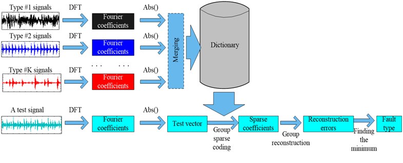
Fig. 1Scheme of the proposed classification method for machinery vibration signals based on group sparse representation
Finally, the category of is labeled based on the minimal reconstruction error:
where , and are the sub-set of the dictionary and coefficient vector associated with class , respectively.
The flowchart of the proposed classification method for machinery vibration signals is shown in Fig. 1, which includes the following main steps:
Step 1: Perform DFT to translate all the vibration signal samples into frequency-domain, including a test sample and training samples;
Step 2: Construct a dictionary with the modulus values of DFT coefficients of the training samples;
Step 3: Project the modulus values of DFT coefficients of the test sample on the dictionary and utilize the algorithm in Table 1 to get group sparse coefficients;
Step 4: Categorize the test sample based on the minimal reconstruction error and determine its fault-type.
5. Performance evaluation
5.1. Simulation analysis
This subsection mainly demonstrates that the proposed method has strong noise immunity and its classification performance is almost unaffected by the sampling starting point. The classification performance includes three factors, i.e. reconstruction errors (RE) (Eq. (19)), SCI (Eq. (20)) [8] and accuracy rate (AR) (Eq. (21)):
Seven types of signals, including a normal signal and six fault signals, are simulated as seven conditions of a rolling element bearing, i.e. no fault, two outer-race faults with different defect sizes, two ball faults with different defect sizes and two inner-race faults with different defect sizes, respectively. The normal signal is set as a white Gaussian noise (WGN) signal with unit standard deviation. For the six fault signals, their model is expressed as:
where denotes amplitude modulation frequency, is attenuation factor, is impulse number, and are natural frequency and fault feature frequency, respectively. These parameters are set as in Table 2. The seven signals with sampling frequency of 2048 Hz are plotted in Fig. 2.
Each of the seven signals is mixed with 50 different WGN keeping SNR in the range of –2 dB to 2 dB such that 350 (50×7) training samples are obtained. The fault 1 signal is chosen as a test object. At first, it is mixed with WGN to get a noisy signal with SNR of 0 dB. After implementation of the proposed method, the sparse coefficients and RE of the noisy signal are obtained (in Fig. 3), both of which confirm that the test sample is of fault 1 category. Then, the WGN intensity is enlarged to reduce SNR to –2 dB and the proposed method is performed as above.
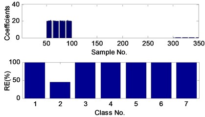
Although the sparse coefficients spread to three classes and the minimal RE magnifies a lot (in Fig. 4), the test sample still can be classified correctly according to the minimal RE, which shows the strong noise immunity of the proposed method. At last, the fault 1 signal with SNR of 0 dB is circularly shifted right 50 points and tested as above. From Fig. 5, it can be seen that the classification performance is almost unaffected by the sampling starting point.
Table 2Parameters of the seven simulation signals
Category | Feature-frequency (Hz) | Modulation-frequency (Hz) | Attenuation-factor |
Normal | – | – | – |
Fault 1 | 14 | 0 | 100 |
Fault 2 | 14 | 0 | 300 |
Fault 3 | 25 | 0.2 | 100 |
Fault 4 | 25 | 0.2 | 300 |
Fault 5 | 20 | 0.1 | 100 |
Fault 6 | 20 | 0.1 | 300 |
Fig. 2The waveform of seven simulation signals, which simulate seven conditions of a rolling element bearing (from above to below: no fault, two outer-race faults with different defect sizes, two ball faults with different defect sizes and two inner-race faults with different defect sizes)
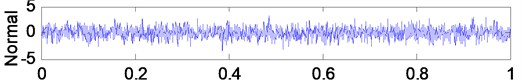
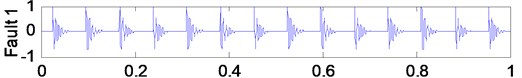
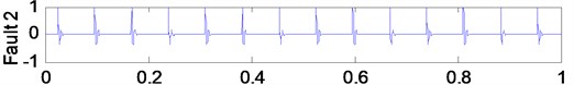
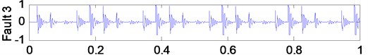
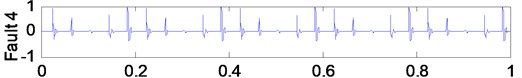
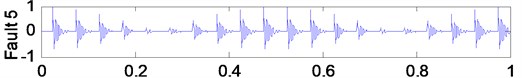
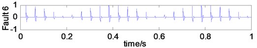
Fig. 3The sparse coefficients and reconstruction errors (RE) of the fault 1 test sample with SNR of 0 dB, obtained by the proposed method
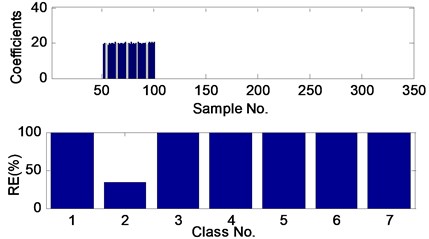
Fig. 4The sparse coefficients and reconstruction errors (RE) of the fault 1 test sample with SNR of –2 dB, obtained by the proposed method
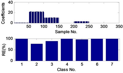
Fig. 5The sparse coefficients and reconstruction errors (RE) of the fault 1 test sample with SNR of 0 dB and circularly shifting right 50 points, obtained by the proposed method
Most tests are conducted. 50 signals of each category with SNR in the range of –2 dB to 2 dB are generated as the test samples. So far, the “simulation dataset”, containing 350 training samples and 350 test ones, has been constructed, which will be used again in discussion section. The proposed method is executed to classify the 350 test samples. The results (summarized in Table 5) preliminarily demonstrate the classification performances of the proposed method.
5.2. Classification results of bearing vibration data
To investigate the effectiveness of the proposed method for vibration signal classification, bearing vibration signals are considered in this subsection.
The vibration dataset from Case Western Reserve University Bearing Data Center [19] has been analyzed by lots of researchers [20-21] and considered as a benchmark. In our study, this dataset is adopted as well. The experimental platform consists of a motor, a dynamometer, a torque transducer, and control electronics. Single point faults of size 0.007, 0.014, 0.021 and 0.028 in. were set on the drive-end bearings (Type 6205-2RS JEM SKF) at the location of outer raceway, inner raceway and rolling element (ball), respectively. The vibration data were measured by using an accelerometer being attached to the motor housing with the sampling frequency of 12 kHz.
In this experiment, twelve fault-types of vibration data are chosen to construct training and test datasets, including a normal, three types of outer race fault, four types of inner race fault, and four types of ball fault. Each data is split with an overlapping length of 512-point into lots of segments, whose length are set to 2048-point. From these segments, we randomly select 50 ones as training samples and other 25 ones as testing samples. Totally, 600 (12×50) samples and 300 (12×25) samples with 12 classes of bearing data are used as training set and test one, respectively. The descriptions of the “bearing dataset” are shown in Table 3.
Table 3Description of bearing dataset for classification
Fault type | Data file | Number of training/testing samples | Label of class |
Normal | Normal_0 | 50/25 | N |
Outer-race | OR007@6_0 | 50/25 | O-I |
Outer-race | OR014@6_0 | 50/25 | O-II |
Outer-race | OR021@6_0 | 50/25 | O-III |
Inner-race | IR007_0 | 50/25 | I-I |
Inner-race | IR014_0 | 50/25 | I-II |
Inner-race | IR021_0 | 50/25 | I-III |
Inner-race | IR028_0 | 50/25 | I-IV |
Ball | B007_0 | 50/25 | B-I |
Ball | B014_0 | 50/25 | B-II |
Ball | B021_0 | 50/25 | B-III |
Ball | B028_0 | 50/25 | B-Ⅳ |
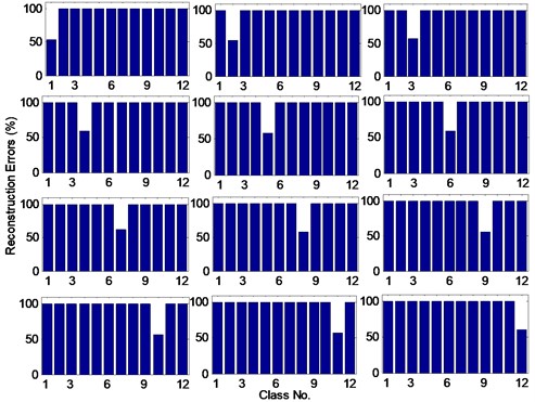
Without loss of generality, we randomly select a test sample from each class and classify them by the proposed method. Their sparse coefficients and RE are plotted in Fig. 6 and Fig. 7, respectively, from which we can see that almost all sparse coefficients of each test sample appear in their own corresponding class and the minimal RE of each test sample just corresponds to its class with value significantly smaller than the other RE. Then, all the 300 test samples are classified by the proposed method. The results (summarized in Table 5), including AR, average SCI and average minimal reconstruction error (AMRE), show that our method can correctly category all the test samples with a high average SCI and relatively low AMRE.
5.3. Classification results of gearbox vibration data
The proposed method is further applied in gearbox fault diagnosis. The experimental platform consists of a motor, a drive shaft seat, a gearbox and a damper, etc. The vibration signals are acquired by an acceleration sensor placed in the output shaft bearing seat. A normal situation and five fault-ones, including three single faults, i.e. tooth-broken and point-corrosion of large gear, wear-out of small gear, and two combination faults, i.e. broken-wear and point-wear faults, are considered. Rotating speed is set as 1500 r/min. The horizontal vibration signals are collected with a sampling frequency of 5120 Hz and the sampling time is about 20 s in each situation.
Fig. 6The sparse coefficients of test samples from each class in bearing dataset
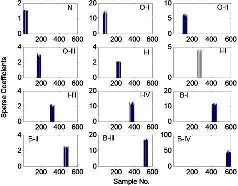
Fig. 7The reconstruction errors of test samples from each class in bearing dataset
Like the experiment of bearing data classification, in the preprocessing stage, each of the six gearbox vibration signals is split with an overlapping length of 128-point into lots of segments, whose length are set to 2048-point. From these segments, we randomly select 50 ones as training samples and other 20 ones as testing samples. Totally, there are 300 (6×50) training samples and 120 (6×20) test samples. The descriptions of the “gearbox dataset” are shown in Table 4.
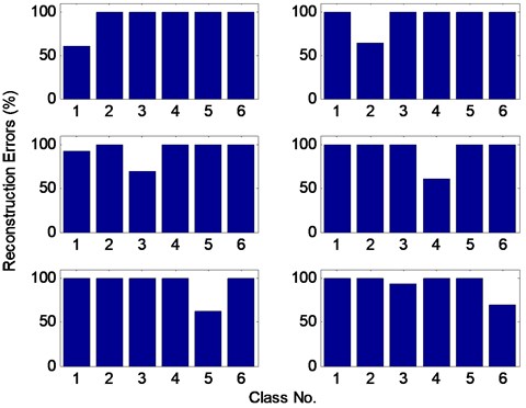
Without loss of generality, we randomly select a test sample from each class and classify them by the proposed method. Their sparse coefficients and RE are plotted in Fig. 8 and Fig. 9, respectively. From Fig. 8, it can be seen that most of sparse coefficients of each test sample appear in their own corresponding class except for “PCL” and “PCL-WOS” samples. The reason for this phenomenon is that the feature frequency of point-corrosion fault is just equal to rotating frequency and the instantaneous value of vibration signal will almost do not change compared with normal conditions when the fault size is little. The minimal RE of each test sample in Fig. 9 indicates the proposed method can correctly classify it.
The classification results of the 120 test samples are displayed in Table 5. The accuracy rate has reached to 97.5 % (117/120), which verifies that our method can be applied in the gearbox fault diagnosis. Moreover, the high average SCI (0.9723) demonstrates again that group sparse representation based classification method can represent a test vibration signal using only signals from the same fault-type.
Table 4Description of gearbox dataset for classification
Fault type | Number of training/testing samples | Label of class |
Normal | 50/20 | N |
Tooth-broken in large gear | 50/20 | TBL |
Point-corrosion in large gear | 50/20 | PCL |
Wear-out in small gear | 50/20 | WOS |
Tooth-broken in large gear and wear-out in small gear | 50/20 | TBL-WOS |
Point-corrosion in large gear and wear-out in small gear | 50/20 | PCL -WOS |
6. Discussions
In this section, we discuss issues from two aspects, i.e. the influence of parameters, and comparison with some other methods.
6.1. The influence of parameters
In our proposed method, two important parameters should be considered. One is the total points of DFT , and the other is the regularization parameter of GSR . In all of the tests above, including simulation analysis and two experiments, is set equally to the length of samples (i.e. ) and is set as 0.5.
Fig. 10 shows the relationship between classification accuracy rate and the total points of DFT. It can be seen that the accuracy rate is improved significantly with the increase of the total points of DFT. Theoretically, the more DFT points, the more spectral information we can get. Therefore, we can improve the accuracy rate by increasing DFT points. However, group sparse representation will need more computational time to complete when the number of DFT point increases. For machinery fault diagnosis, vibration signal is analyzed in real-time and diagnostic conclusion should be determined in the crucial early hours. This requires the computational time of a diagnosis method as shorter as possible. As far as the proposed method, it needs to balance the classification accuracy rate and computational time to determine DFT points. In general, we can set DFT points as the half of sample length if accuracy rate is in range of acceptance.
Fig. 8The sparse coefficients of test samples from each class in gearbox dataset
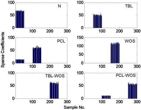
Fig. 9The reconstruction errors of test samples from each class in gearbox dataset
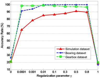
The relationship between classification accuracy rate and the regularization parameter is visualized in Fig. 11, which demonstrates that the accuracy rate almost keeps unchanged with a high value when the parameter varies in [0.0001, 0.8], while the accuracy rate will drop sharply if approaches to 0 or 1. In other words, when group sparse representation are utilized in classification of machinery vibration signals, the influence of the regularization parameter is very limited when it is set in a reasonable range.
Besides and , the termination tolerance and sample length have some effect on the classification results as well. In all of the tests above, and is set respectively as 0.001 and 2048. From Table 1, it can be seen that directly determines the runtime of coefficient solving algorithm and the reconstruction error. For classification-based diagnosis method, the reconstruction precision is not as important as for other signal approximation problems. Therefore, we set the termination condition of coefficient solving algorithm as the difference of objective function of two adjacent iterations less than to reduce runtime. The parameter has similar effect with on classification accuracy rate and computational time. In practical application, if the training samples of each class are enough, a time-series vibration signal should no longer be split into a number of segments unless its length is too long. In this case, should be regulated rather than .
Fig. 10The accuracy rate of the three datasets with the change of DFT points N
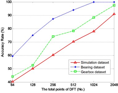
Fig. 11The accuracy rate of the three datasets with the change of regularization parameter γ
6.2. Comparison of the proposed method with some other methods
In this subsection, the proposed method is compared with SRC and SVM to demonstrate its superiority.
The L1-norm based SRC [8] is utilized to classify the test samples of three datasets for comparison. It is known there have been many effective methods for solving L1-minimization problems. Here, l1ls [20], SLEP [17] and GPSR [23] are adopted respectively to solve the problem. From the results in Table 5, it is seen that their classification performances are not as good as that of the proposed method. Specifically, AR and average SCI obtained by the three methods are respectively lower than that of proposed method roughly 10 and 50 percent, while average minimal RE is higher 20 percent or so.
For further comparison, the three datasets are tested by SVM method. SVM is a pattern recognition classification algorithm indicating favorable generalization performance based on statistical learning theory [24]. Fault classifications are achieved with these methods as characteristic parameters (e.g., root mean square value, kurtosis, mean square frequency, etc.) from time and frequency domains are extracted and adjusted based on the actual situation [5]. Modeled on reference [25], vibration signals are translated into different frequency bands by wavelet package transform (WPT); then, the optimal features are selected based on the distance evaluation technique from the statistical characteristics of raw signals and wavelet package coefficients, and the energy characteristics of decomposition frequency band, finally, the optimal features are input the SVM ensemble with SVM toolbox [26] to identify the fault type. The results recorded in Table 5 show that the AR obtained by the SVM ensemble method is improved significantly compared with that of SRC, yet it is still lower than that of the proposed method.
Table 5Classification results of the three datasets obtained by the proposed method and other methods
Method | Simulation dataset | Bearing dataset | Gearbox dataset | |||||||||
AR (%) | ASCI | AMRE (%) | CT (s) | AR (%) | ASCI | AMRE (%) | CT (s) | AR (%) | ASCI | AMRE (%) | CT (s) | |
l1ls-SRC | 76.3 | 0.354 | 87.2 | 23.2 | 91.0 | 0.287 | 84.5 | 30.4 | 88.6 | 0.284 | 81.6 | 19.4 |
SLEP-SRC | 80.2 | 0.387 | 89.3 | 10.3 | 90.6 | 0.417 | 86.2 | 19.6 | 84.3 | 0.453 | 80.5 | 8.5 |
GPSR-SRC | 84.3 | 0.401 | 86.5 | 11.2 | 91.0 | 0.413 | 86.2 | 20.4 | 86.5 | 0.412 | 84.6 | 9.6 |
SVM ensemble | 91.9 | – | – | 79.5 | 98.7 | – | – | 146.3 | 96.4 | – | – | 69.8 |
Proposed method | 93.4 | 0.894 | 69.5 | 10.9 | 100 | 0.99 | 58.6 | 21.6 | 97.5 | 0.97 | 63.3 | 9.4 |
AR: accuracy rate; ASCI: average sparsity concentration index; AMRE: average minimal reconstruction error; CT: computational time | ||||||||||||
In machinery fault diagnosis, classification efficiency is another important factor. We investigate the computational time (CT) of these methods on the three datasets and tabulate the results in Table 5. Matlab 2012b is run with a computer of CPU: 3.6 GHz, RAM: 4G. From the observations, the proposed method is as fast as SRC solved by SLEP and GPSR and significantly faster than SVM ensemble and SRC solved by l1l s.
7. Conclusions
This paper presents a new classification method based on group sparse representation for machinery vibration signals. In the method, time-domain vibration signals are transformed into Fourier coefficients by DFT at first; then, the transform coefficient vectors of the training samples are merged as a dictionary and the transform coefficient vectors of the test samples are coded on the dictionary by group sparse representation algorithm; finally, the class labels of the test samples are identified by the minimal reconstruction error. Simulation analysis has shown that the proposed method has a strong noisy immunity and its classification performance is almost unaffected by the sampling starting point. The classification results of bearing and gearbox vibration signals demonstrate the method can effectively diagnose both of them fault types with a high accuracy and efficiency.
References
-
Harris F. J. Rolling Bearing Analysis 2. John Wiley, New York, 2000.
-
Shin Younghak, Lee Seungchan, Ahn Minkyu, et al. Noise robustness analysis of sparse representation based classification method for non-stationary EEG signal classification. Biomedical Signal Processing and Control, Vol. 21, 2015, p. 8-18.
-
Rafiee J., Tse P. W., Harifi A., et al. A novel technique for selecting mother wavelet function using an intelligent fault diagnosis system. Expert Systems with Applications, Vol. 36, 2009, p. 4862-4875.
-
Wang D., Tse P. W., Tsui K. L. An enhanced kurtogram method for fault diagnosis of rolling element bearings. Mechanical Systems and Signal Processing, Vol. 35, 2013, p. 176-199.
-
Tang G., Yang Qin, Wang Hua-Qing, et al. Sparse classification of rotating machinery faults based on compressive sensing strategy. Mechatronics, 2015, (in Press).
-
Qi Zhiquan, Tian Yingjie, Shi Yong Robust twin support vector machine for pattern classification. Pattern Recognition, Vol. 46, 2013, p. 305-316.
-
Huang K., Aviyente S. Sparse representation for signal classification. Advances in Neural Information Processing Systems, Vol. 19, 2006, p. 609-616.
-
Wright John, Yang Allen Y., Ganesh Arvind, et al. Robust face recognition via sparse representation. IEEE Transactions on Pattern Analysis and Machine Intelligence, Vol. 31, Issue 2, 2009, p. 210-227.
-
Chen S., Donoho D. L., Saunders M. A. Atomic decomposition by basis pursuit. SIAM Journal on Scientific Computing, Vol. 20, 1998, p. 33-61.
-
Zhang D., Yang M., Feng X. Sparse representation or collaborative representation: which helps face recognition? IEEE International Conference on Computer Vision (ICCV), 2011, p. 471-478.
-
Zhang Xin, Pham Duc-Son, Venkatesh Svetha, et al. Mixed-norm sparse representation for multi view face recognition. Pattern Recognition, Vol. 48, 2015, p. 2935-2946.
-
Majumdar A., Ward R. K. Classification via group sparsity promoting regularization. IEEE International Conference on Acoustics, Speech and Signal Processing, 2009, p. 861-864.
-
Sheng Huang, Yu Yang, Dan Yang, et al. Class specific sparse representation for classification. Signal Processing, Vol. 116, 2015, p. 38-42.
-
Roth V., Fischer B. The group-lasso for generalized linear models: uniqueness of solutions and efficient algorithms. International Conference on Machine Learning, 2008, p. 848-855.
-
Qin Z., Scheinberg K., Goldfarb D. Efficient block-coordinate descent algorithms for the group lasso. Mathematical Programming Computation, Vol. 5, Issue 2, 2013, p. 143-169.
-
van den Berg E., Schmidt M., Friedlander M., Murphy K. Group Sparsity Via Linear-Time Projection. Computer Science department at the University of British Columbia, Vancouver, BC, Canada, 2008.
-
Liu J., Ji S., Ye J. SLEP: Sparse Learning with Efficient Projections. Arizona State University, 2009.
-
Liu J., Ye J. Efficient L1/Lq-norm Regularization. Technical Report, Arizona State University, 2009.
-
Case Western Reserve University Bearing Data Center Website. http://csegroups.case.edu/bearingdatacenter/home.
-
He Qingbo Vibration signal classification by wavelet packet energy flow manifold learning. Journal of Sound and Vibration, Vol. 332, 2013, p. 1881-1894.
-
Smith Wade A., Randall Robert B. Rolling element bearing diagnostics using the Case Western Reserve University data: a benchmark study. Mechanical System and Signal Processing, Vols. 64-65, 2015, p. 100-131.
-
Kim S.-J., Koh K., Lustig M., Boyd S., Gorinevsky D. A method for large-scale L1-regularized least squares. IEEE Journal on Selected Topics in Signal Processing, Vol. 1, Issue 4, 2007, p. 606-617.
-
Figueiredo Mario A. T., Nowak Robert D., Wright Stephen J. Gradient projection for sparse reconstruction: application to compressed sensing and other inverse problems. Journal of Selected Topics in Signal Processing: Special Issue on Convex Optimization for Signal Processing, 2007.
-
Cristianini N., Shawe-Taylor J. An Introduction to Support Vector Machines and Other Kernel-Based Learning Methods. Cambridge University Press, Cambridge, UK, 2000.
-
Hu Qiao, He Zhengjia, Zhang Zhousuo, et al. Fault diagnosis of rotating machinery based on improved wavelet package transform and SVMs ensemble. Mechanical Systems and Signal Processing, Vol. 21, 2007, p. 688-705.
-
Chang C. C., Lin C. J. LIBSVM: A Library for Support Vector Machines. Software available at: http://ntucsu.csie.ntu.edu.tw/~cjlin/libsvm/, 2001.
Cited by
About this article

This work is partially supported by the National Natural Science Foundation of China (No. 61174106) and the Key Scientific Research Project of Education Department of Henan Province (No. 15B510017)
