On the conditions for synchronous harmonic free vibrations

Morales, César A.

Journal of Vibroengineering

Browse Journal

Submit article

Published: 15 November 2015

Check for updates

On the conditions for synchronous harmonic free vibrations

César A. Morales¹

¹Departamento de Mecánica, Universidad Simón Bolívar, Apdo. 89000, Caracas 1080A, Venezuela

Cite the article Download PDF

Downloads 1190

Abstract

All conditions for synchronic harmonic oscillations are presented. These are for discrete and continuous undamped linear systems in free vibration. A vibrations literature review indicates that only one or the basic condition for synchronous harmonic free vibrations is known. This is, initial conditions as an eingenvector (or eigenfunction) for the initial displacements, and no generalized velocities for $t = 0$ . Moreover, although assumed or expected for continuous systems, this result appears solely or mainly for discrete systems in the literature.

1. Introduction

It is known that if a linear conservative system is imparted initial conditions as: 1) a mode shape for the initial displacements, and 2) no velocities for $t =$ 0, the ensuing oscillation will be harmonic and synchronous. Mathematically, the mode is an eigenvector or an eigenfuction, and the frequency $ω$ of this special motion is the square root of the corresponding eigenvalue, or the natural frequency [1]. Nonetheless, this basic result does not appear in most books on the subject of linear mechanical vibrations [2-6], even in the case of an $n$ -degree-of-freedom discrete system; other than [1], the result is presented by [7] but for the particular and hypothetical case of a particle elastically supported in 3 dimensions, in [8] but for the proportional damping case which implies that the motion is synchronous but not harmonic, and by [9] but only for 2-degree-of-freedom systems. In the case of distributed systems, the presentation of the result is even rarer.

Regarding synchronous nonharmonic vibrations in discrete systems, Felszeghy presented a comprehensive work [10] including both, proportional damping and classical damping [11]. The oscillations were called “synchronous damped harmonic”, and the conditions for the synchronous motion were on the system damping rather than on the initial conditions. On the other hand, Wilms presented a highly symmetric damped system for which it is shown that the oscillation of each body is at the same and only “damped” frequency found in the work [12]. However, these vibrations for that special and hypothetical system are neither synchronous nor harmonic.

Herein, the conditions on initial conditions for synchronic harmonic oscillations in discrete and continuous linear conservative systems are presented, in free vibration of course. Moreover, the expressions for all these special responses are presented as well.

2. Conditions for synchronous harmonic free vibration in discrete systems

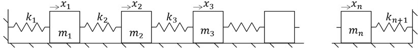
The equations of free motion of an $n$ -degree-of-freedom undamped vibratory system, such as the one shown in Fig. 1, are:

1

M \ddot{q} + K q = 0,

where $M$ is the mass matrix, $K$ is the stiffness matrix and $q$ is the vector of generalized coordinates, or the system response; however, the straight-through system of Fig. 1 is just an example, the system can also be branched. The associated eigenvalue problem is normally written as:

2

K u = λ M u,

whose solutions are n eigenvalues $λ_{r} = ω_{r}^{2}$ , and $n$ mode shapes $u_{r}$ which are orthogonal through both, the mass matrix and the stiffness matrix; this implies after the correct normalization that:

3

u_{i}^{T} M u_{j} = δ_{i j}, u_{i}^{T} K u_{j} = δ_{i j} ω_{i}^{2},

where $δ_{i j}$ is the Kronecker delta. Now, the general free response of the system is given by:

4

q (t) = \sum_{r = 1}^{n} (u_{r}^{T} M q (0) \cos ω_{r} t + u_{r}^{T} M \dot{q} (0) \frac{1}{ω_{r}} \sin ω_{r} t) u_{r},

where $ω$ are the natural frequencies [1].

As previously explained, a review on free vibrations of mechanical systems indicates that only the first or basic case has been reported regarding the question of which initial conditions imply synchronous harmonic oscillations. That is, it is known that if the initial conditions are such that the initial displacements resemble an eigenvector, and the initial generalized velocities are null, or $q (0) = q_{o} u_{s}$ and $\dot{q} (0) = 0$ , the ensuing motion is given by:

5

q (t) = q_{o} u_{s} \cos ω_{s} t,

which is absolute and perfect synchronous harmonic vibration; this can be considered Case 1, for the conditions to have this special type of motion.

Fig. 1Discrete undamped vibratory system

2.1. Case 2

Now, it is also possible to experience harmonic and synchronous oscillations if $q (0) = 0$ and $\dot{q} (0) = v_{o} u_{s}$ ; that is, if the initial displacement vector is zero whereas the initial velocity vector is a normal mode, except for a constant velocity factor. This can be proved by substituting these initial conditions in Eq. (4):

6

q (t) = \sum_{r = 1}^{n} (\frac{v_{o}}{ω_{r}} u_{r}^{T} M u_{s} \sin ω_{r} t) u_{r},

and by considering the orthogonality of mode shapes, or the first part of Eq. (3); the response is simply:

7

q (t) = \frac{v_{o}}{ω_{s}} u_{s} \sin ω_{s} t .

This is also perfect and absolute synchronic harmonic oscillations, at natural frequency $ω_{s}$ ; the system configuration at all times resembles the corresponding mode $s$ .

2.2. Case 3

Furthermore, if the system is provided an initial displacement in its sth mode shape and the initial velocities resemble the same eigenvector, or $q (0) = q_{o} u_{s}$ and $\dot{q} (0) = v_{o} u_{s}$ , the response is again harmonic and synchronous, or:

8

q (t) = (q_{o} \cos ω_{s} t + \frac{v_{o}}{ω_{s}} \sin ω_{s} t) u_{s},

which can be finally simplified to:

9

q (t) = A u_{s} \cos (ω_{s} t - φ),

where $A$ and $φ$ are constants that depend only on the initial-condition factors $q_{o}$ and $v_{o}$ , as:

10

φ = \tan^{- 1} \frac{v_{o}}{q_{o} ω_{s}}, A = \frac{q_{o}}{\cos φ} .

In spite of the phase angle $φ$ , the response in Eq. (9) is perfectly harmonic and synchronous as well.

2.3. Cases 4A and 4B

Moreover, assuming that $q (0) = q_{o} A u_{s}$ and $\dot{q} (0) = 0$ , and that matrix $A$ is either $M^{- 1} K$ (case 4A) or $K^{- 1} M$ (case 4B), the response or Eq. (4) becomes:

11

q (t) = \sum_{r = 1}^{n} (q_{o} u_{r}^{T} M M^{- 1} K u_{s} \cos ω_{r} t) u_{r},

for the first subcase, and:

12

q (t) = \sum_{r = 1}^{n} (q_{o} u_{r}^{T} M K^{- 1} M u_{s} \cos ω_{r} t) u_{r},

for the second one. Considering the other orthogonality or the second part of Eq. (3) in Eq. (11), and considering:

13

u_{r}^{T} M K^{- 1} = \frac{1}{ω_{r}^{2}} u_{r}^{T},

(which is derived from Eq. (2)) in Eq. (12), the ensuing motions finally are synchronic and harmonic, respectively:

14

q (t) = q_{o} ω_{s}^{2} u_{s} \cos ω_{s} t,

15

q (t) = \frac{q_{o}}{ω_{s}^{2}} u_{s} \cos ω_{s} t .

Matrix $A$ is commonly known as the dynamic matrix in case 4A [2, 9], and as dynamical matrix in case 4B [13].

Nevertheless, cases 4A and 4B are not of much interest because multiplication of the dynamic matrix, or the dynamical matrix, by an eigenvector, results in the same mode shape, as can be concluded by premultiplying the eigenproblem or Eq. (2) by the inverse of the inertia matrix, and the inverse of the stiffness matrix, respectively:

16

M^{- 1} K u = λ u,

17

K^{- 1} M u = \frac{1}{λ} u .

In other words, cases 4A and 4B are similar or equivalent to case 1. Therefore, cases 5 and 6 with initial conditions $q (0) = 0$ and $\dot{q} (0) = v_{o} {A u}_{s}$ , and $q (0) = q_{o} A u_{s}$ and $\dot{q} (0) = v_{o} {A u}_{s}$ will not be pursued.

3. Examples of synchronous harmonic vibrations in lumped-parameter systems

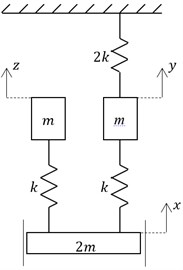
The three degree-of-freedom system of Fig. 2 will be used to illustrate cases 2 and 3. If $m =$ 10 kg and $k =$ 1000 N/m, it is undergraduate level to find the natural frequencies and corresponding orthonormal eigenvectors:

18

ω_{1} = 4.45 rad / s, ω_{2} = 12.47 rad / s, ω_{3} = 18.02 rad / s,

19

u_{1} = {(0.165 0.059 0.206)}^{T},

u_{2} = {(0.132 0.091 - 0.238)}^{T},

u_{3} = {(0.073 - 0.297 - 0.033)}^{T} .

Fig. 2Example discrete system

3.1. Case 2

If $q (0) = {(0 0 0)}^{T}$ m, and $\dot{q} (0) = {(1 0.692 - 1.8)}^{T}$ m/s, then:

20

u (t) = (\begin{matrix} 0.080 \\ 0.055 \\ - 0.144 \end{matrix}) \sin 12.47 t .

Every body has the same harmonic motion, except for the amplitude; also, there is no phase angle except for the fact that the third body is –perfectly– out of phase with respect to the first two bodies, which are in phase. Of course, the vibrations would be in perfect phase if we had chosen the first mode as initial velocities. More interestingly, the amplitudes of vibration are proportional to the initial velocities.

3.2. Case 3

If $q (0) = {(0.165 0.059 0.206)}^{T}$ m, and $\dot{q} (0) = {(1 0.357 1.25)}^{T}$ m/s:

21

q (t) = (\begin{matrix} 0.279 \\ 0.099 \\ 0.347 \end{matrix}) \cos (4.45 t - 0.938) .

Again, all masses have the same harmonic motion, and reach their maximum, and minimum, displacement at the same time; the ratios of these amplitudes are the same as the eigenvector ratios. There is no relative phase angle.

4. Conditions for synchronous harmonic free vibration in distributed systems

The general equation of free vibration of a continuous undamped system is:

22

L [w (x, y, t)] + m \frac{\partial^{2} w (x, y, t)}{\partial t^{2}} = 0 .

Above, $L$ is a linear homogeneous self-adjoint differential operator of order 2 $p$ [6, 13], that is related to the distributed stiffness of the system or body, $m$ is the constant mass density, and $w$ is of course the displacement or system response. This general analysis includes uniform strings, rods in axial and torsional vibration, beams, membranes and plates. At all boundary points we have $p$ boundary conditions to be satisfied therein and of the type:

23

B_{i} [w (x, y, t)] = 0,

where $B$ is a linear homogeneous differential operator of order less than 2 $p -$ 1. Note that for strings and rods or bars, there are only two boundary points with only one condition per point; for beams there are two conditions per end ( $i =$ 1, 2); moreover, for these systems there is only one spatial coordinate $x$ .

The associated differential eigenvalue problem over domain $D$ can be written as:

24

L [w (x, y)] = ω^{2} m w (x, y),

the eigenproblem includes the boundary conditions:

25

B_{i} [w (x, y)] = 0 .

The eigensolution are infinite but countable natural frequencies $ω_{r}$ , and corresponding mode shapes or eigenfunctions $w_{r}$ , which are orthogonal; if the mass distribution is uniform as assumed, the orthogonality can be written as:

26

\int_{D}^{} w_{r} w_{s} d D = 0, r \neq s,

which implies after the correct normalization that:

27

m \int_{D}^{} w_{r} w_{s} d D = δ_{r s}, \int_{D}^{} w_{r} L [w_{s}] d D = ω_{r}^{2} δ_{r s} .

It is noted that if the mass density is a function $m (x)$ or $m (x, y)$ , the orthogonality of eigenfunctions still holds, even the second part of Eq. (27) fully holds; constant mass density is assumed herein just to simplify the mathematics and because it is most common in engineering to design with uniform mass distribution. An actual constant-density differential eigenvalue problem is presented in [14].

Now, the general free response of the distributed system is given by:

28

w (x, y, t) = \sum_{r = 1}^{\infty} w_{r} (x, y) (η_{r} (0) \cos ω_{r} t + \frac{1}{ω_{r}} {\dot{η}}_{r} (0) \sin ω_{r} t),

where the initial modal displacements and velocities are given by [13]:

29

η_{r} (0) = m \int_{D}^{} w_{r} (x, y) w (x, y, 0) d x d y, {\dot{η}}_{r} (0) = m \int_{D}^{} w_{r} (x, y) \dot{w} (x, y, 0) d x d y,

in terms of the initial deformation and initial actual velocities.

We are in search for all initial conditions that result in perfect harmonic and synchronous vibrations in one and two dimensional distributed systems.

4.1. Case 1

Let us assume that the initial conditions are such that the initial displacements of the continuous body resemble a mode shape or eigenfunction, and that the initial velocities are null, or $w (x, y, 0) = w_{o} w_{s} (x, y)$ and $\dot{w} (x, y, 0) = 0$ ; it follows from Eqs. (28) and (27) that:

30

w (x, y, t) = w_{o} w_{s} (x, y) \cos ω_{s} t .

This is absolute and perfect synchronous harmonic vibration, at natural frequency $ω_{s}$ ; the system configuration at all times resembles the corresponding mode $s$ , and each point mass oscillates harmonically in perfect phase with the other points.

4.2. Case 2

In a continuum, it should also be possible to experience harmonic and synchronous oscillations if $w (x, y, 0) =$ 0 and $\dot{w} (x, y, 0) = v_{o} w_{s} (x, y)$ ; that is, if the initial displacements are zero whereas the initial velocity function is a normal mode, except for a constant velocity factor. A proof can be established by substituting these initial conditions into Eq. (28):

31

w (x, y, t) = \sum_{r = 1}^{\infty} w_{r} (x, y) (\frac{1}{ω_{r}} m \int_{D}^{} v_{o} w_{r} (x, y) w_{s} (x, y) d x d y \sin ω_{r} t),

and by considering the first part of Eq. (27) of course, which implies:

32

w (x, y, t) = \frac{v_{o}}{ω_{s}} w_{s} (x, y) \sin ω_{s} t .

This is also perfect and absolute distributed synchronic harmonic oscillation, every point mass has the same harmonic motion except for the amplitude, and there is no phase angle except for $π$ for some points that may not be considered as a phase. It is interesting to note the similarity between responses Eqs. (7) and (32), or the similarity in dynamical characteristics exhibited by discrete and continuous systems: the only difference in the response is a vector instead of a function, but this is no difference as distributed and lumped-parameter systems represent merely distinct mathematical models of identical physical systems.

4.3. Case 3

Moreover, if the system is provided an initial deformation in its sth mode and the initial velocities resemble the same eigenfunction, or $w (x, y, 0) = w_{o} w_{s} (x, y)$ and $\dot{w} (x, y, 0) = v_{o} w_{s} (x, y)$ , the response is again harmonic and synchronous, or:

33

w (x, y, t) = w_{s} (x, y) (w_{o} \cos ω_{s} t + \frac{v_{o}}{ω_{s}} \sin ω_{s} t),

which can be finally simplified to:

34

w (x, y, t) = A w_{s} (x, y) \cos (ω_{s} t - φ),

where $A$ and $φ$ are constants that depend solely on the initial-condition factors $w_{o}$ and $v_{o}$ , as:

35

φ = \tan^{- 1} \frac{v_{o}}{w_{o} ω_{s}}, A = \frac{w_{o}}{\cos φ} .

In spite of the phase angle $φ$ , the response in Eq. (34) is perfectly synchronous and harmonic as well.

5. Examples of synchronous harmonic vibrations in distributed-parameter systems

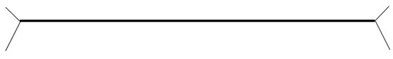
The uniform string of Fig. 3 is used to illustrate cases 4.2 and 4.3; it can be a beam with more diverse supports (or boundary conditions) and the development will be very similar, but the string is far more intuitive than a beam, or a rod, membrane or plate for that matter. If $m =$ 10 kg/m, and the tension along the string (of length 1 m) is $T =$ 1000 N, it is graduate level to find the natural frequencies: $ω = 10 π r,$ or $ω_{1} =$ 31.42 rad/s, $ω_{2} =$ 62.83 rad/s, $ω_{3} =$ 94.25 rad/s, and corresponding orthonormal eigenfunctions, which have only one spatial or independent variable in this case:

36

w_{r} (x) = 5^{- 1 / 2} \sin r π x .

Fig. 3Uniform string

5.1. Case 2

If $w (x, 0) =$ 0 and $\dot{w} (x, 0) = \sin 3 π x$ ( $v_{o} = \sqrt{5}$ m/s), the response is:

37

w (x, t) = 0.0106 \sin 3 π x \sin 94.2 t .

Again, all mass points have the same harmonic motion, and all reach their maximum (or minimum) displacement at the same time; moreover, if a picture is taken at any time, the third mode will always be observed.

5.2. Case 3

Finally, if $w (x, 0) = \sin π x$ and $\dot{w} (x, 0) = 5 \sin π x$ ( $w_{o} = \sqrt{5}$ m, $v_{o} =$ 11.18 m/s), the synchronous harmonic distributed vibration is:

38

w (x, t) = 1.01 \sin π x \cos (31.4 t - 0.159) .

In other words, every point mass moves as:

39

w (t) = a \cos (31.4 t - 0.159),

and at every instant the deformation is:

40

w (x) = b \sin π x .

This is, we believe, the best way to explain what synchronous harmonic vibration is.

6. Conclusions

Until now, only one or the basic condition for synchronous harmonic free vibrations was known: initial conditions as an eingenvector (or eigenfunction) for the initial displacements, and no generalized velocities for $t =$ 0; furthermore, although assumed or expected for continuous systems, this result appears only or mainly for discrete systems in the Vibrations literature.

We have presented all conditions for synchronic harmonic oscillations in both, discrete and distributed mechanical systems. It is concluded that there are two additional (new) and significant initial conditions that imply this special motion: a mode shape as initial velocities, and an eigen vector or function as initial deformation and the same mode shape as initial velocities. Moreover, the expressions for all these synchronic-harmonic responses are presented, and examples are provided for selected and interesting cases. The results are for linear and undamped systems of course.

References

Meirovitch L. Elements of Vibrations Analysis. McGraw-Hill, Mexico, 1986.

Search CrossRef
Thomson W. T., Dahleh M. D. Theory of Vibration with Applications. Prentice-Hall, USA, 1998.

Search CrossRef
Rao S. S. Mechanical Vibrations. Prentice-Hall, USA, 2011.

Search CrossRef
Dimarogonas A. D. Vibration for Engineers. Prentice-Hall, USA, 1996.

Search CrossRef
Steidel R. F. An Introduction to Mechanical Vibrations. John Wiley and Sons, USA, 1989.

Search CrossRef
Meirovitch L. Principles and Techniques of Vibrations. Prentice-Hall, USA, 1997.

Search CrossRef
Timoshenko S., Young D. H. Vibration Problems in Engineering. Van Nostrand, USA, 1955.

Search CrossRef
Balachandran B., Magrab E. B. Vibrations. Thomson, USA, 2004.

Search CrossRef
Chen Y. Vibrations: Theoretical Methods. Addison-Wesley, USA, 1966.

Search CrossRef
Felszeghy S. F. The development of natural modes of free vibration for linear discrete system from synchronous motion assumption. Journal of Vibration and Acoustics, Vol. 111, 1989, p. 77-81.

Search CrossRef
Caughey T. K., O’Kelly M. E. J. Classic normal modes in damped linear dynamic systems. Journal of Applied Mechanics, Vol. 32, 1965, p. 583-588.

Search CrossRef
Wilms E. V. The motion of a damped n-degree-of-freedom system with a single natural frequency. Journal of Sound and Vibration, Vol. 204, 1997, p. 679-680.

Search CrossRef
Meirovitch L. Analytical Methods in Vibrations. Macmillan, USA, 1967.

Search CrossRef
Morales C. A., Goncalves R. Eigenfunction convergence of the Rayleigh-Ritz-Meirovitch method and the FEM. Shock and Vibration, Vol. 14, 2007, p. 417-428.

Search CrossRef

About this article

Received

15 April 2015

Accepted

15 July 2015

Published

15 November 2015

SUBJECTS

Modal analysis

Keywords

free vibration

synchronous harmonic motion

conditions

Acknowledgements

This work was supported by Decanato de Investigación, Universidad Simón Bolívar, Grant No. S1-IC-CAI-018-14.

This is an open access article distributed under the Creative Commons Attribution License, which permits unrestricted use, distribution, and reproduction in any medium, provided the original work is properly cited.