Abstract
Model reduction of large-scale structures has been improved and a weight coefficient reflecting the contribution proportion of a higher-order model has been introduced contribution based on the shortcomings of conventional optimization algorithms, with the aim to solve the problem that conventional optimization algorithms do not serve the optimized distribution of large-scale structure observation stations. Therefore, two hybrid optimization algorithms are proposed based on the effective independence method. The effective independence-average modal kinetic/strained energy coefficient methods have been compared with effective independence method for Guyan reduction based on modal kinetic/strained coefficients and the respectively improved ones through a GARTEUR plane simulation experiment. Results have shown that both of the two algorithms effectively avoided the emergence of concentrated observation stations, best ensured the contribution of all modal kinetic and strain energy and the requirements that the better-arranged observation station has much more strained energy. Model tests were also made on the two methods by employing real GARTEUR plane, which showed that the two algorithms guaranteed the completeness and linear independence of monitoring mode and that the two are of great practical value to the observation station optimization and distribution of large-scale structures.
1. Introduction
Vibration testing technique analyzes the dynamic responses of structures after collecting data through modal tests. If the optimization scheme of observation stations is not properly adopted, the collected data will be incomplete or inaccurate. Coupled with expensive sensors and their accessories, (of large-scale complex structures in particular), the vibration test will be highly costly. Considering economic costs and the practicality, we must carry out the test with the fewest sensors to obtain the most complete and accurate data. Hence, how to manage a best optimization scheme of observation tests is of great study and application value.
At the very beginning, the sites and number of observation stations are dependent on the tester’ experience and his knowledge of the characteristics of the dynamic responses of structures. Without scientific methods to determine the sites and number of sensors, the resultant measurement will be inaccurate. In recent years, scientists from home and abroad have begun to introduce some advanced algorithms to the field of observation station optimization and done a lot of research. Presently, the observation station optimization can generally be divided into non-traditional conventional and conventional optimization algorithms, the former including wavelet method, particle swarm algorithm, artificial neural networks analysis and genetic algorithm [2] and the latter including minimum MAC algorithm [3], effective independence method [4, 5], Guyan reduction method [6, 7], energy method [8, 9] etc.
Each and every optimization algorithm has its advantages and limitations [9] and application scopes. In terms of large-scale complex structures, their modal information that is quite important will be lost and optimization tarnished if only one algorithm is used due to their highly distinct vibration mode and liberal computing.
Consequently, this work proposes two hybrid optimization algorithms based on the effective independence method. First, the thesis, through the improved model reduction technique, simplifies the model by removing the unnecessary, uninfluential or fixed aspects, followed by a weight coefficient reflecting the contribution proportion of a higher-order model to best ensure that the requirements that the better-arranged observation station has much more strained energy. Finally, the structural model of the GARTEUR plane is taken as an engineering example and observation optimization and distribution are done on it. The modal test of GARTEUR plane proves that the two hybrid optimization algorithms based on the effective independence method mentioned here can well be applied.
2. Optimization lay-out theory and its evaluation criteria
2.1. Effective independence method
The most widely used algorithm is EI (Effective Independence method), proposed by Kammer [10], from which many other algorithms have evolved. Its core idea is to remove those observation stations that contribute the least to the target linearly -independent mode to make the determinant of the Fisher matrix [11] that corresponds to the remaining ones get the maximum value. In the matrix, represents the inherent mode of former S-order, thus ensuring that the resultant modes of the remaining observation stations are the best evaluated.
Matrix of EI goes as follows:
where represents feature vector of matrix Fisher and represents the corresponding feature value while equals to the total of coefficients. represents the linearly-independent contribution of a given observation station to a target modal vibration mode.
2.2. Modal kinetic energy method and strain energy method
The sensor arrangement of modal kinetic energy method and modal strain energy method [12, 13] is similar to that of effective independence method. The main difference lying in that in the case of the former, the observation station is set where the modal kinetic and strain energy reach the highest, rather than being decided by the maximum determinant of Fisher matrix. To sum up, the principle obeyed in applying the two methods to select the optimal observation station is that the kinetic and strain energy must peak wherein.
The modal kinetic and strain energy can be expressed as follows:
where represents modal matrix and target modal value. The greatest strength of the modal kinetic energy method and modal strain energy method is that they work well even in adverse environment.
2.3. Mode assurance code
Values of inherent modal vibration modes of structures form a set of orthogonal vectors on nodes. But it is impossible that the number of observation stations is equivalent to that of nodes. Instead, the number of nodes is far larger. That is even truer for large and complex structures. Jointed by measurement accuracy and the effects of noise, the orthogonality of target modal vibration modes measured cannot be ensured. Therefore, in selecting observation stations, it is necessary to retain the completeness of dynamic characteristics of the structural models and to ensure broad intersect angle between modes to its best.MAC (Mode assurance code) matrix [3] gives a fair orthogonal evaluation on the modal vectors and can be expressed as follows:
In the equation, and are respectively -order and -order modal vectors. Whether the two corresponding mode shapes are orthogonal can be judged by examining the non-diagonal element of MAC matrix of each mode within the freedom degree of measuring. When MAC is less than 0.25, the two vectors are generally believed to be mutually orthogonal; when MAC is greater than 0.9, the two vectors are believed to be relevant.
3. Hybrid optimization algorithms based on the effective independence method
With the increasingly higher requirements on model computing (especially of large and complex structure), freedom degrees of one hundred thousand or even one million are quite common. If these magnitudes are introduced into the observation station, the computing will be troublesome or even cannot be conducted. However, the mode reduction technique can effectively solve the problem by removing unnecessary, uninfluential and fixed freedom degrees and simplifies modes by choosing influential and needed ones. Guyan mode reduction technique ignores the inertia amount but it is only when the mass that corresponds to the reduced freedom degree is extremely small can the error be left out. Hence, the structural inertia amount cannot be ignored in terms of large-scale structures. This work improves this and deduces a series of scientific, accurate and rigorous formula.
Conventional methods believe that the mode strain energy is mainly concentrated in low-order modes and that high-order modes contribute little to the energy. But for large and complex structures, their contribution to the mode strain energy cannot be ignored. This paper presents a weight coefficient [15] reflecting the contribution of high-order modes, which not only meet the requirements that the selected observation station has much more strained energy but also take into consideration the contribution of modes of all orders.
3.1. Reduction improvement
Suppose that the stiffness matrix of a system with n degree of freedom is , mass matrix and characteristic pair and (), the vibration mode can be expressed as follows:
where represents the column vector derived from the measuring coordinate of a vibration mode and the column vector of a reduced coordinate. Correspondingly, the characteristic equation of the structural vibration is expressed as:
From the second part of Eq. (6), we can infer:
To unfold Eq. (7) according to Neumann series, we may get:
where “” represents an extremely small high order. To omit the high order of Eq. (8), we may arrive at:
From the first part of Eq. (6) we can also infer:
For the finite model of most structures, the mass matrix is usually diagonal matrix. Hence, we come to:
To substitute Eq. (10) into Eq. (9), we may get:
To substitute Eqs. (11) and (12) into Eq. (9), we may get:
From Eq. (13), we may infer:
Therefore, the improved reduced equation is expressed as:
where the transformation matrix is:
To substitute Eqs. (15) and (13) into Eq. (5), we may arrive at:
If both sides of Eq. (17) time we may arrive at:
Suppose that:
We may get:
To substitute Eq. (9) into Eq. (20), we may get:
Therefore, the reduced characteristic equation is expressed as:
3.2. Weight coefficient
For large-scale structures, due to highly distinct vibration distribution of modes, the contribution of high-order modes to the modal strain energy cannot be ignored. In order to cover the contribution to the strain energy of all modes and improve the accuracy of the result, we come up with a weight coefficient reflecting the contribution of high-order modes to amend the matrix of modal vibration modes. The weigh coefficient is calculated under:
where represents the frequency of -order and weight coefficient of -order.
3.3. Optimization method
The selection of an observation station when applying mode kinetic energy method and made strain energy is decided by the total energy of all target modes at the station, which will lead to information loss of some target modes due to uneven energy distribution of orders in large and complex structures. To tackle this dilemma, guided by the two methods mentioned here, we select observation station according to the average modal kinetic and strain energy coefficients of each station.
3.3.1. Effective independence-average modal kinetic energy coefficient method
From the Eq. (2), we may infer the modal kinetic energy coefficient of the th freedom degree at th order, namely:
Then, we may get he average modal strain energy coefficient of the the freedom degree is:
To combine the Eq. (1) with Eq. (28), we may arrive at the effective independence method based on average kinetic energy coefficient:
3.3.2. Effective independence-average modal strain energy coefficient method
From the Eq. (3), we may infer the modal strain energy coefficient of the th freedom degree at th order, namely:
Then, the average modal strain energy coefficient is:
To combine Eq. (2) and (31), we may get the effective independence method based on average strain energy coefficient as follows:
After the iterative calculation of and , we may choose the observation station that corresponds to the maximum of and until that the maximum value of non-diagonal elements of MAC matrix that corresponds to all the selected stations is eligible. In order to avoid concentrated stations, we need to check that whether the distances between this station and all other selected one are longer than and , which are already smallest. Herein:
There-into, is a constant, representing the smallest distance appointed. That the areas with greater structural vibration are equipped with more sensors and vice versa will not only ensure the completeness and independence of the target modes but also avoid concentrated stations.
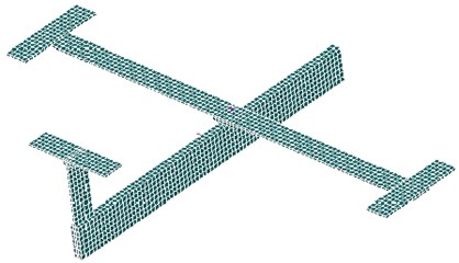
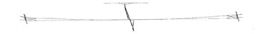
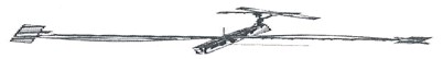
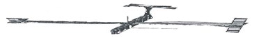
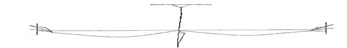
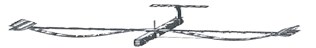
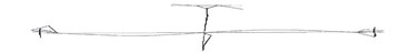
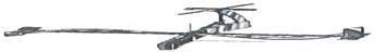
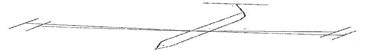
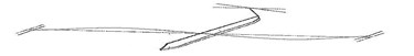
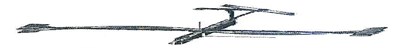
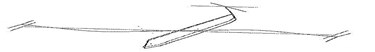
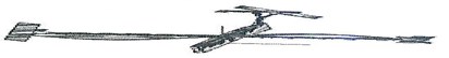
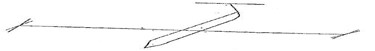
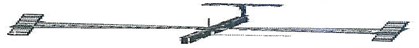
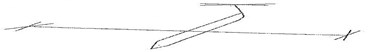
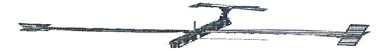
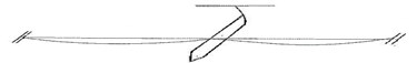
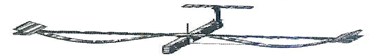
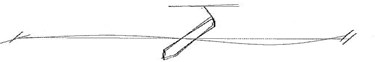
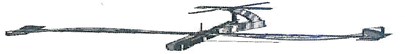
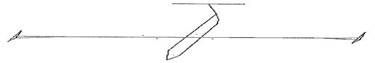
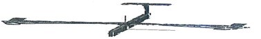
Fig. 1The plane model
4. Simulation example
4.1. About the model
In conducting the experiment of observation station arrangement optimization, a GARTEUR plane model was applied. As is shown in Fig. 1, the model has 2640 cells and 5106 nodes, hence, 30636 freedom degrees. Modal vibration of the plane is mainly , and -directed, so the 3 rotational freedom degrees can be designated as ancillary ones, which makes the follow-up optimization calculating much easier. Material parameters of plane models: the elastic modulus is 7 E10 Pa, Poisson’s ratio of 0.3 and material density 2800 Kg/m3.
To take the modes of first 15 orders as target vibration modes and their inherent frequency is shown in Table 1.
Table 1Inherent frequency of the first 15 orders (Unit: Hz)
Order | 1 | 2 | 3 | 4 | 5 | 6 | 7 | 8 |
Frequency | 6.0914 | 16.601 | 36.973 | 37.577 | 37.67 | 48.757 | 49.183 | 56.919 |
Order | 9 | 10 | 11 | 12 | 13 | 14 | 15 | |
Frequency | 65.363 | 73.818 | 97.034 | 137.41 | 143.65 | 159.05 | 229.03 |
4.2. Observation station arrangement optimization and comparison
a) Sensor arrangement of effective independence method for Guyan reduction based on modal kinetic/strained coefficients and the respectively improved ones and effective independence-average modal kinetic/strained energy coefficient methods are compared as is shown in Fig. 2.
1) Fig. 2(a) Guyan-reduction average modal kinetic energy coefficient effective-independence method and Fig. 2(d) Guyan-reduction average modal strained energy coefficient effective-independence method give rise to relatively concentrated sensor placement. In other words, these sensors are unevenly distributed and some of them are even sitting together. In this way, some modal information will be obtained repeatedly while some other important modal information will be lost. We can see that the resultant observation stations of these two methods entail many sensors. As a result, high economic costs will be caused during collection tests of modal data and the experiment will be complicated, thereby being not conducive to the modal data collection. In a word, both of the two are undesirable.
2) Fig. 2(a) improved-reduction average modal kinetic energy coefficient effective-independence method and Fig. 2(d) Improved-reduction average modal strained energy coefficient effective-independence method, however, will give rise to relatively disperse sensor placement. Sensors are evenly distributed and the number of observation stations are smaller. Consequently, economic costs caused during collection tests of modal data will be lowered and the experiment will turn easier. Compared with the methods Fig. 2(a) and Fig. 2(b), these two methods not only largely reduce the number of observation stations but also bring about evener and more reasonable sensor placement. It is fair to say that to improve reduction, to some extent, renders the model more concise and faithful. Thus, these two discussed here are favorable.
3) Fig. 2(c) effective independence-average modal kinetic energy coefficient method and Fig. 2(f) effective independence-average modal strained energy coefficient method proposed in this paper actually bring about rather even senor placement and a fairly small quantity of observation stations. Hence, the modal information will not be lost and the economic costs will be reduced by a large margin. Moreover, the experiment will become even easier. Among Fig. 2(a), (d), (b), (e), (c) and (f), the latter two methods turn out to be the optimal ones in that they allow the fewest observation stations, best sensor placement, lowest economic costs of tests and easiest experiment. It can be concluded hereby that weight coefficients play a positive role in the remedying of high-order targeted modes of vibration. In summary, the two sensor placement optimization schemes put forward in this paper are the best, both in terms of the number and positions of sensors coupled by the fact that they best retain the real structures under test and complete dynamic characteristics.
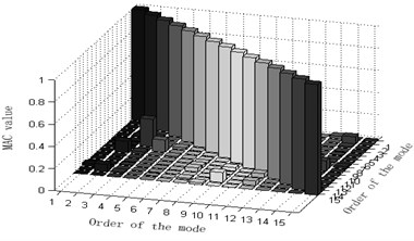
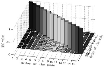
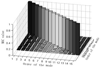
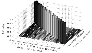
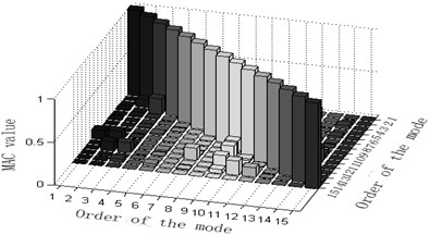
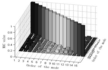
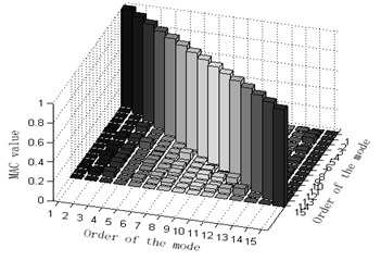
b) Column graphs of MAC matrix obtained from the six mentioned optimization algorithm are shown in Fig. 3.
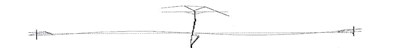
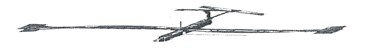
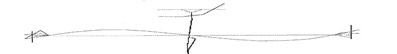
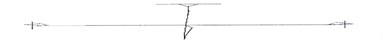
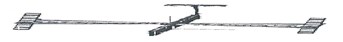
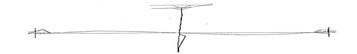
Fig. 2Sensor arrangement of varied methods
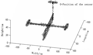
a) Guyan-reduction average kinetic energy coefficient effective-independence method (Number of needed observation stations: 82)
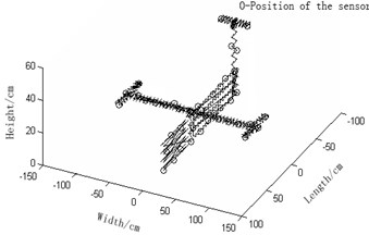
b) Improved-reduction average kinetic energy coefficient effective-independence method (Number of needed observation stations: 44)
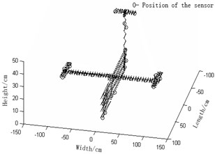
c) Effective independence-average modal kinetic energy coefficient method (Number of needed observation stations: 34)
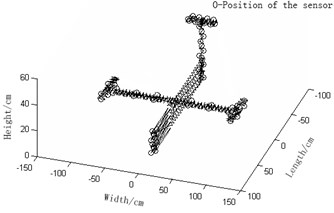
d) Guyan-reduction average modal strain energy coefficient effective-independence method (Number of needed observation stations: 79)
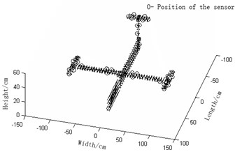
e) Improved-reduction average modal strain energy coefficient effective-independence method (Number of needed observation stations: 42)
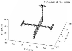
f) Effective independence -average modal strain energy coefficient method (Number of needed observation stations: 33)
The maximum value of non-diagonal element of MAC matrix is an important index to judge whether target modal vibration modes are relevant or not. When MAC is less than 0.25, the two vectors are generally believed to be mutually orthogonal; when MAC is greater than 0.9, the two vectors are believed to be relevant. Judging the Fig. 3, one can see that: 1) part of the non-diagonal element values of MAC matrix derived from methods Fig. 3(a) and (d) are somewhat great, indicating that the orthogonality between the targeted modes of vibration is unsatisfactory and that Fig. 3(a) and (d) are not ideal schemes. 2) The non-diagonal element values of MAC matrix derived from methods Fig. 3(b) and (e) are relatively small and a lot smaller than those from Fig. 3(a) and (d). Thus, the orthogonality between the targeted modes of vibration of Fig. 3(b) and (e) are good and better than that of Fig. 3(a) and (d), implying that Fig. 3(b) and (e) are better schemes than Fig. 3(a) and (f). Methods Fig. 3(c) and (f) proposed in this paper results in quite small non-diagonal element values of MAC matrix that are almost zero. Right here, one may conclude that the resultant orthogonality is much preferable than Fig. 3(a), (d), (b) and (e) and that weight coefficients are beneficial to the remedying of high-order targeted modes of vibration. Therefore, Fig. 3(c) and (f) are the soundest sensor placement optimization schemes.
By comparing the results of the six different sensor arrangement scheme, we may infer that the effective independence – average modal kinetic/strain energy coefficient methods not only maintain the maximum linear- independence of target modes and genuine and complete dynamic characteristics if the observed modes but also avoid the loss of information of high-order modes at the low-energy, being the most reliable and effective one among the six optimization algorithms.
Fig. 3Column diagram of MAC matrix in applying varied methods
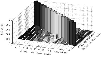
a) Guyan-reduction average kinetic energy coefficient effective-independence method
b) Improved-reduction average kinetic energy coefficient effective-independence method
c) Effective independence-average modal kinetic energy coefficient method
d) Guyan-reduction average modal strain energy coefficient effective-independence method
e) Improved-reduction average modal strain energy coefficient effective-independence method

f) Effective independence -average modal strain energy coefficient method
5. Simulation experiment
GARTEUR airplane model is a typical standard aircraft developed by the European Aviation Technology Research Organization Structures and Materials Working Group that has 12 members, characteristic of the density, high flexibility and low modal frequency of a real aircraft. Having model it using Patran and simulated it with the hybrid optimization methods here, we may get an optimization scheme, conduct a modal experiment and finally compare the resultant parameters with the ones obtained from simulation tests. Devices and analysis software applied in the modal test:
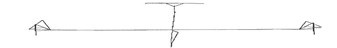
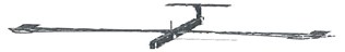
1) Suspension: Use elastic ropes and detailed suspension points are shown in Fig. 4.
2) One hammer and one PCB acceleration sensor, sensor fixation: the super glue 502, the arrangement of observation stations is seen in Fig. 4, run-point test mode is applied.
3) Data-collecting platform and software: the platform is the USB-4431 data collected of NI; signal collecting and analyzing software is NJSamp.
4) Software for modal analysis: NJModal.
The observation station arrangement of the sensors and the establishment of the experimental platform are shown in Fig. 4.
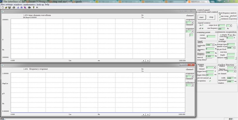
The interface of the Software NJSamp collecting and analyzing signals is shown in Fig. 5.
Fig. 4The observation station arrangement of the sensors and the establishment of the experimental platform
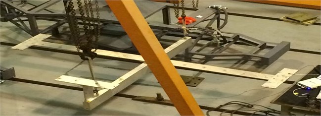
Fig. 5The interface of the Software NJSamp collecting and analyzing signals
5.1. Effective independence – average modal kinetic energy coefficient method
The experiment is to test the resultant scheme of the effective independence-average modal kinetic energy coefficient method proposed in this paper. The optimized placement of observation stations hereby is the optimized placement Fig. 2(c) among all methods in Fig. 2.
a) Coordinate –based locations of sensor placement (Table 2).
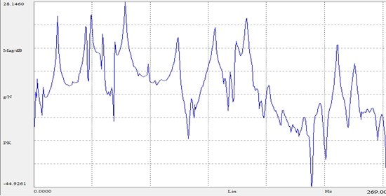
b) Frequency response function logarithmic curve shown in Fig. 6.
c) Comparison and contrast between experiment frequency and simulation frequency (Table 3).
d) The comparison and contrast of MAC matrix orthogonal graphs is shown in Fig. 7.
e) The comparison and contrast of the vibration modes of the first experimented 8 orders and simulation vibration modes is shown in Fig. 8.
Table 2Coordinate – based locations of sensor placement
Number of observation stations | Coordinate | Number of observation stations | Coordinate | ||||
1 | –8.50e+01 | –2.00e+01 | 4.50e+01 | 18 | –8.50e+01 | 6.35e+00 | 4.60e+01 |
2 | –8.50e+01 | 2.00e+01 | 4.50e+01 | 19 | 0.00e+00 | 8.52e+01 | 1.66e+01 |
3 | –2.00e+01 | 9.52e+01 | 1.76e+01 | 20 | 0.00e+00 | –8.52e+01 | 1.66e+01 |
4 | –2.00e+01 | –9.52e+01 | 1.76e+01 | 21 | –8.00e+01 | 5.00e–01 | 3.74e+01 |
5 | 2.00e+01 | –9.52e+01 | 1.76e+01 | 22 | 5.50e+01 | 2.10e+00 | 1.00e+01 |
6 | 2.00e+01 | 9.52e+01 | 1.76e+01 | 23 | 5.00e+00 | 9.52e+01 | 1.88e+01 |
7 | 0.00e+00 | 4.04e+01 | 1.66e+01 | 24 | 5.00e+00 | –9.52e+01 | 1.88e+01 |
8 | 0.00e+00 | –4.04e+01 | 1.66e+01 | 25 | 6.00e+01 | 2.10e+00 | 0.00e+00 |
9 | 0.00e+00 | –7.03e+01 | 1.66e+01 | 26 | –9.00e+01 | 5.00e–01 | 3.18e+01 |
10 | 0.00e+00 | 7.03e+01 | 1.66e+01 | 27 | –8.50e+01 | 5.00e–01 | 1.50e+01 |
11 | –5.00e+00 | 1.00e+02 | 1.76e+01 | 28 | –1.00e+01 | –9.02e+01 | 1.88e+01 |
12 | –5.00e+00 | –1.00e+02 | 1.76e+01 | 29 | –1.00e+01 | 9.02e+01 | 1.88e+01 |
13 | 0.00e+00 | 5.53e+01 | 1.66e+01 | 30 | 4.50e+01 | 2.10e+00 | 0.00e+00 |
14 | 0.00e+00 | –5.53e+01 | 1.66e+01 | 31 | –9.00e+01 | 5.00e–01 | 5.00e+00 |
15 | 0.00e+00 | –2.54e+01 | 1.66e+01 | 32 | 4.50e+01 | 2.10e+00 | 1.50e+01 |
16 | 0.00e+00 | 2.54e+01 | 1.66e+01 | 33 | –1.50e+01 | 2.10e+00 | 0.00e+00 |
17 | –8.50e+01 | –6.35e+00 | 4.60e+01 | 34 | –5.00e+00 | –2.10e+00 | 0.00e+00 |
Table 3Experiment frequency and simulation frequency
Order | Experiment frequency / Hz | Simulation frequency / Hz | Error % |
1 | 6.0225 | 6.0914 | 1.131 |
2 | 15.9722 | 16.601 | 3.788 |
3 | 35.5273 | 36.973 | 3.910 |
4 | 38.3159 | 37.577 | 1.967 |
5 | 39.4961 | 37.67 | 4.848 |
6 | 46.7549 | 48.757 | 4.106 |
7 | 46.9038 | 49.183 | 4.634 |
8 | 55.0728 | 56.919 | 3.244 |
9 | 62.4173 | 65.363 | 4.507 |
10 | 73.4862 | 73.818 | 0.449 |
11 | 98.6483 | 97.034 | 1.664 |
12 | 138.542 | 137.41 | 0.824 |
13 | 145.102 | 143.65 | 1.010 |
14 | 159.992 | 159.05 | 0.592 |
15 | 229.354 | 229.03 | 0.141 |
Fig. 6Frequency response function logarithmic curve
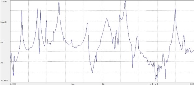
Fig. 7Comparison and contrast of MAC matrix orthogonal graphs
a) Experimented MAC matrix orthogonal graph

b) Simulated MAC matrix orthogonal graph
Fig. 8The comparison and contrast of the vibration modes of the first experimental 8 orders and simulation vibration modes
a) Experimented vibration mode of the 1st order

b) Simulated vibration mode of the 1st order
c) Experimented vibration mode of the 2nd order
d) Simulated vibration mode of the 2nd order
e) Experimented vibration mode of the 3rd order
f) Simulated vibration mode of the 3rd order
g) Experimented vibration mode of the 4th order
h) Simulated vibration mode of the 4th order
i) Experimented vibration mode of the 5th order
j) Simulated vibration mode of the 5th order
k) Experimented vibration mode of the 6th order
l) Simulated vibration mode of the 6th order
m) Experimented vibration mode of the 7th order
n) Simulated vibration mode of the 7th order
o) Experimented vibration mode of the 8th order
p) Simulated vibration mode of the 8th order
5.2. Effective independence – average modal kinetic energy coefficient method
The experiment is to test the resultant scheme of effective independence-average modal strained energy coefficient method proposed in this paper. The optimized placement of observation stations hereby is the optimized placement Fig. 2(f) among all methods in Fig. 2.
a) Coordinate – based locations of sensor placement (Table 4).
b) Frequency response function logarithmic curve shown in Fig. 9.
c) Comparison and contrast between experiment frequency and simulation frequency (Table 5).
d) The comparison and contrast of MAC matrix orthogonal graphs is shown in Fig. 10.
e) The comparison and contrast of the vibration modes of the first experimented 8 orders and simulation vibration modes is shown in Fig. 11.
Table 4Coordinate – based locations of sensor placement
Number of observation stations | Coordinate | Number of observation stations | Coordinate | ||||
1 | –8.50E+01 | –2.00E+01 | 4.50E+01 | 18 | –9.00E+01 | 5.00E–01 | 3.18E+01 |
2 | –8.50E+01 | 2.00E+01 | 4.50E+01 | 19 | –8.50E+01 | 5.00E–01 | 1.50E+01 |
3 | –2.00E+01 | 9.52E+01 | 1.76E+01 | 20 | –9.00E+01 | –6.35E+00 | 4.60E+01 |
4 | –2.00E+01 | –9.52E+01 | 1.76E+01 | 21 | –9.00E+01 | 6.35E+00 | 4.60E+01 |
5 | 2.00E+01 | –9.52E+01 | 1.76E+01 | 22 | 5.50E+01 | 2.10E+00 | 1.00E+01 |
6 | 2.00E+01 | 9.52E+01 | 1.76E+01 | 23 | –8.50E+01 | –5.00E–01 | 0.00E+00 |
7 | 0.00E+00 | 4.04E+01 | 1.66E+01 | 24 | 6.00E+01 | 2.10E+00 | 0.00E+00 |
8 | 0.00E+00 | –4.04E+01 | 1.66E+01 | 25 | 5.00E+00 | 8.02E+01 | 1.66E+01 |
9 | 0.00E+00 | 7.03E+01 | 1.66E+01 | 26 | 5.00E+00 | –8.02E+01 | 1.66E+01 |
10 | 0.00E+00 | –7.03E+01 | 1.66E+01 | 27 | 5.00E+01 | –2.10E+00 | 0.00E+00 |
11 | 0.00E+00 | 9.52E+01 | 1.76E+01 | 28 | 4.50E+01 | 2.10E+00 | 1.50E+01 |
12 | 0.00E+00 | –9.52E+01 | 1.76E+01 | 29 | 5.00E+00 | 1.55E+01 | 1.66E+01 |
13 | –8.00E+01 | –5.00E–01 | 4.30E+01 | 30 | 5.00E+00 | –1.55E+01 | 1.66E+01 |
14 | 5.00E+00 | 5.53E+01 | 1.76E+01 | 31 | 4.00E+01 | 2.10E+00 | 5.00E+00 |
15 | 5.00E+00 | –5.53E+01 | 1.76E+01 | 32 | –1.50E+01 | 2.10E+00 | 0.00E+00 |
16 | 0.00E+00 | –2.54E+01 | 1.66E+01 | 33 | –2.50E+01 | –2.10E+00 | 0.00E+00 |
17 | 0.00E+00 | 2.54E+01 | 1.66E+01 | ||||
Table 5Experiment frequency and simulation frequency
Order | Experiment frequency / Hz | Simulation frequency / H | Error % |
1 | 6.010 | 6.0914 | 1.336 |
2 | 16.064 | 16.601 | 3.235 |
3 | 35.771 | 36.973 | 3.251 |
4 | 37.687 | 37.577 | 0.293 |
5 | 39.222 | 37.67 | 4.120 |
6 | 46.886 | 48.757 | 3.837 |
7 | 47.063 | 49.183 | 4.310 |
8 | 55.347 | 56.919 | 2.762 |
9 | 62.384 | 65.363 | 4.558 |
10 | 72.023 | 73.818 | 2.432 |
11 | 98.796 | 97.034 | 1.816 |
12 | 138.923 | 137.41 | 1.101 |
13 | 146.301 | 143.65 | 1.845 |
14 | 160.435 | 159.05 | 0.871 |
15 | 229.875 | 229.03 | 0.369 |
Fig. 9Frequency response function logarithmic curve
By examining the experiments and simulation tests of the two methods proposed in the paper, we may see: differences between the experiment frequency and simulation experiment of both methods are small and simulation frequencies, which are less than five percent; MAC orthogonal graphs of each experiment and simulation test are quite similar and each vibration modes are orthogonally convergent; modal vibration modes of each experiment and simulation test are in agreement. Then, the two hybrid optimization methods proposed here may serve good guidance to the observation station optimization of large-scale structure se and are of great practical value.
Fig. 10Comparison and contrast of MAC matrix orthogonal graphs
a) Experimented MAC matrix orthogonal graph
b) Simulated MAC matrix orthogonal
Fig. 11The comparison and contrast of the vibration modes of the first experimented 8 orders and simulation vibration modes
a) Experimented vibration mode of the 1st order

b) Simulated vibration mode of the 1st order
c) Experimented vibration mode of the 2nd order
d) Simulated vibration mode of the 2nd order
e) Experimented vibration mode of the 3rd order
f) Simulated vibration mode of the 3rd order
g) Experimented vibration mode of the 4th order
h) Simulated vibration mode of the 4th order
i) Experimented vibration mode of the 5th order
j) Simulated vibration mode of the 5th order
k) Experimented vibration mode of the 6th order
l) Simulated vibration mode of the 6th order
m) Experimented vibration mode of the 7th order
n) Simulated vibration mode of the 7th order
o) Experimented vibration mode of the 8th order
p) Simulated vibration mode of the 8th order
6. Conclusion
Comparing and contrast of the aforesaid six methods through GARTEUR airplane simulation experiments show that both of the two hybrid algorithms proposed in the paper effectively avoided the emergence of concentrated observation stations and ensured the contribution of all modal kinetic and strain energy and best ensured the contribution of all modal kinetic and strain energy and the requirements that the better-arranged observation station has much more strained energy.
Modal parameters obtained from the experiments on these two methods through the use of GARTEUR airplane and those from simulation tests show that the two algorithms both guaranteed the completeness and linear-independence of the observed modes and of great practical value to the observation station optimization and distribution of large-scale structures by solving the problem that conventional algorithms fail to do so.
The main strengths of the algorithm are as follows:
a) Due to the fact that the conventional Guyan reduction method ignores the inertial amount of structures, great errors will happen in the case of the large-massed reduced freedom degrees. the proposed improved reduction method takes into consideration the first-order inertial amount of structures, significantly enhancing accuracy.
b) The introduction of weight coefficient not only brings into play the modal kinetic and strain energy in arranging observation stations but also keep unchanged the important information of target modes of all orders.
c) Making the maximum value MAC of non-diagonal elements that corresponds to the selected observation stations less than 0.1 the convergent threshold will manage the calculation of number and coordinate positions of optimal observation stations, which other algorithms cannot do.
References
-
Dai Jiangbo, Ji Guoyi Parameter recognition of GARTEUR airplane models. Noise and Vibration Control, Vol. 33, Issue 3, 2013, p. 73-78.
-
Wu Ziyan, Jian Xiaohong, Zhang Bin on distribution optimization of multi-target sensors in vibration tests. Mechanical Strength, Vol. 30, Issue 6, 2008, p. 888-892.
-
Dai Hang, Yuan Aimin Structural Mode Amendment Based on Sensitivity Analysis (First Edition). Science Press, Beijing, 2001, p. 215.
-
Kammer D. C. Sensor placement for on-orbit modal identification and correlation of large space structures. Journal of Guidance, Control, and Dynamic, Vol. 14, Issue 2, 1991, p. 251-259.
-
Kammer D. C., Yao L. Enhancement of on-orbitmoda identification of large space structures throughsensor placement. Journal of Sound and Vibration, Vol. 171, Issue 1, 1994, p. 119-140.
-
Liao Boyu, Zhou Xinmin, Yin Zhihong Modern Mechanical Dynamics and Its Engineering Application. Mechanical Industry Press, Beijing, 2003, p. 701.
-
Guyan R. J. Reduction of stiffness and mass matrices. AIAA Journal, Vol. 3, 2, p. 1965-380.
-
Zumpano Meo G. on the optimal sensor placement techniques for a bridge structure. Engineering Structures, Vol. 27, 2005, p. 1488-1497.
-
Swann Cynthia, Chattopadhyay Sditi Optimization of piezoelectric sensor location for delamination detection in composite laminates. Engineering Optimization, Vol. 38, Issue 5, 2006, p. 511-528.
-
Kammer D. C., Brillhart R. D. Optimal sensor placement for modal identification using system-realization methods. Journal of Guidance, Control, and Dynamic, Vol. 19, 1996, p. 729-731.
-
Worden K., Burrows A. P. Optimal sensor placement for fault detection. Engineering Structures, Vol. 23, 2001, p. 885-901.
-
Klein A., Melard G., Spreij P. On the resultant property of the Fisher information matrix of a vector ARMA process. Linear Algebra and Its Applications, Vol. 403, Issues 1-3, 2005, p. 291-313.
-
Liu Wei, Gao Weicheng, Li Hui, Sun Yi on methods of optimizing sensor distribution based on effective independence algorithm. Vibration and Shock, Vol. 32, Issue 6, 2013, p. 54-62.
-
Yang Qiuwei, Liu Jike an improved modal reduction method. Mechanics and Practice, Vol. 28, Issue 2, 2006, p. 70-72.
-
Wu Ziyan, He Yin, Jian Xiaohong on optimized sensor distribution based on damage sensitivity analysis. Engineering Mechanics, Vol. 26, Issue 5, 2009, p. 239-244.
-
Chern A. P. Optimal sensor placement for modal parameter identification using signal subspace correlation techniques. Mechanical Systems and Signal Processing, Vol. 17, Issue 2, 2003, p. 361-378.
-
Yang YaXun, Hao Hongwu, Sun Lei Optimized sensor distribution of bridge structures based on energy coefficient-effective independence method. Vibration and Shock, Vol. 29, Issue 11, 2010, p. 119-123+134.
-
Tian Ye, Ling Ling, Hu Yujin on optimized distribution of large sensors in dynamic tests. Mechanics and Electronics, Vol. 6, 2013, p. 16-20.
About this article

