Abstract
A novel non-visual vibration shape reconstruction method based on orthogonal curvilinear net is proposed in paper for shape detection and reconstruction of plate structure. Its iteration process is deduced and analyzed. A high precision experimental verification platform is constructed. Real time experiments are done for pure bending deformation, torsional deformation and dynamic vibration. Reconstruction precision and performance is compared with the modal approach using displacement-strain transformation techniques. Experimental results show that the proposed method and the modal approach have good shape reconstruction performance for the static deformation with large amplitude and dynamic low frequency vibration. The reconstruction precision of the proposed algorithm was higher than modal approach for deformation with small amplitude. But the modal approach is better for dynamic high frequency vibration. The reconstruction efficiency of the proposed algorithm is superior to the modal approach.
1. Introduction
Plate structure is a basic component that widely used in aerospace vehicles. Real-time accurate shape reconstruction of plate structure plays an important role in maintaining the healthy operation of aerospace vehicles [1-4]. There are two kinds method for shape reconstruction: vision method [5-8] and non-visual method [9-14]. As non-visual reconstruction method has many advantages, including small amount data needed to acquire, and high acquisition precision, it has become a research hotspot.
Current non-visual shape reconstruction methods for plate structure include modal approach based on strain data [15, 16] and geometric iterative method based on curvature information [17-20]. Modal approach uses displacement-strain transformation techniques. Reference [15, 16] implemented and verified the effectiveness and feasibility of modal approach. But reference [15] only reconstructed the shape of cantilever beam. Reference [16] did not analyze the reconstruction precision of large deformation and computation time performance.
The geometric iterative method can be divided into two algorithms: curved surface reconstruction algorithm based on curvilinear array [17, 18] and curved surface reconstruction algorithm based on patch array [19, 20]. The curved surface reconstruction algorithm using plane curve array only can apply in pure bending deformation, and for more complex torsional deformation, the reconstruction performance is poor. While the curved surface algorithm based on patch array need to solve the complex nonlinear equations, it is difficult to apply in actual systems.
In this paper, a new spatial surface reconstruction algorithm based on orthogonal curvilinear net is proposed. A high precision experimental verification platform is constructed. Real time experiments are done for pure bending deformation, torsional deformation and dynamic vibration under the same experimental condition.
2. Principle and configuration of FBG sensors
2.1. Strain/curvature detection principle of FBG sensors
When the flexible plate structure deformation occurs, the surface would generate a strain. If the impact of environmental temperature changes is ignored, the strain detected by FBG sensors bonded on the structure surface can be considered as strain of the flexible plate structure on the measuring point. When FBG is under longitudinal stretching or compression in elastic range, the performance can be defined as:
where is the axial strain, is the original center wavelength, and is the effective photoelastic coefficient of the fiber. Then, the variation of wavelength is:
The strain sensitivity coefficient of FBG sensor can be defined as:
Then:
where, is constant. The variation of wavelength has a linear relationship with its axial strain. If the value of FBG center wavelength is known, the coefficient can be calculated. should be determined by calibration when it is used in practical application.
In this paper, the experimental model is a plate structure fixed on one end. The FBG sensors bonded on the positive surface is responsible for measuring the longitudinal strain, and the FBG sensors bonded on the negative surface is responsible for measuring the transversal strain. A tiny structural unit, whose length and thickness are and respectively, is selected along the direction of strain measurement. When a pair of bending moments is applied in the unit, the tiny structural unit deformed and curvature radius is , as shown in Fig. 1. In the elastic range, the inner part of the unit is compressed and the outer part of the unit is prolonged. There is a strain neutral layer: its length is unchanged and strain is zero, as the dotted line shown in Fig. 1. Therefore, the curvature of neutral layer can be used to represent shape change of the tiny structural unit. For homogeneous isotropic materials, the strain neutral layer is the physical middle layer in the thickness direction.
Fig. 1Deformation of a tiny structural unit
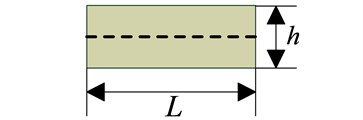
a) Before deformation
b) After deformation
Fig. 1(a) and Fig. 1(b) are the shapes of tiny structural unit before deformation and after deformation respectively. From Fig. 1:
Then, the curvature:
In Eq. (6), is the strain. Combining with Eq. (4):
For a given FBG sensor and a flexible structure, the thickness and strain sensitivity coefficient in Eq. (7) are constant. Therefore, the change of surface curvature has the linear relationship with wavelength.
2.2. Configuration of FBG sensors
Before designing the FBG sensor network, the quantity of sensors on each channel should be determined firstly, and then determine the total number of FBG sensors according to the number of channels in fiber grating network analyzer. Assumed that there are sensors on one single optical fiber, and the strain sensitivity coefficient and the buffer sizes of wavelength on each sensor are the same. In order to avoid the overlapping of sensor wavelength, the measuring range of sensors can be expressed as:
where is strain on measuring point. And the maximum value of the demodulator with non-overlapping spectrum must be satisfied by:
Then:
So:
If the strain range of each sensor measured is , then the Eq. (11) can be simplified as:
The quantity of FBG sensors on each channel can be calculated by Eq. (12). In actual calculation, the limit strain is 2000×106, 0.5 nm and 1.13 pm/10-6. As wavelength measurement range of the instrument is 1530 nm-1570 nm, then is 40 nm. Substituting these parameters into Eq. (12), we can get , which means that 8 FBG points can be set up on each optical fiber. Considering a total of eight channels due to the instrument, the number of FBG sensors on the entire network are 64.
3. Modal approach
3.1. Natural frequency and inherent vibration mode
The motion equations are given by:
where, is the mass matrix; is the damping matrix; is the stiffness matrix; is the load vector and is the displacement vector.
Ignoring damping, and the load vector is zero. The freedom vibration equation is:
Vibration equation of structure is defined by:
where, is -order vector; is the vibration frequency of ; is time variable; is a time constant which is determined by initial condition.
Substituting Eq. (15) into Eq. (14), a generalized eigenvalue problem can be obtained in Eq. (16):
where, the eigenvalues , ,…, (0 ) and eigenvectors , ,…, represent natural modal frequencies and intrinsic modal shape of the system, respectively.
3.2. Displacement-strain-transformation
Since displacement can be regarded as linear combination of inherent mode (1, 2,…, ), a transformation can be introduced:
where represents displacement mode shapes matrix whose size is ×, and represents the modal coordinates. is the number of displacements (the number of finite element nodes), and is the number of modes used.
Similarly, the strain can be defined by Eq. (18):
where, is strain mode shapes matrix whose size is ×, and is the number of strain measures (the number of sensors). When , is not a square matrix. Eq. (19) can be obtained by multiplying on the left and right of the Eq. (18):
Then:
Substituting Eq. (20) into Eq. (17), we obtain:
Displacement-strain-transformation (DST) matrix can be constructed:
Then:
When , the whole displacement of structure can be reconstructed by measuring few nodes’ strain.
4. Curved surface reconstruction algorithm based on orthogonal curvilinear net
The basic process of curved surface reconstruction algorithm based on orthogonal curvilinear net is as follows: constructing the orthogonal curvilinear net by using continuous curvature, and establishing the orthogonal moving coordinate system on two directions for orthogonal curvilinear net; calculating node coordinates of orthogonal curvilinear net using the moving coordinate system, and using the internal relations of different nodes to implement the coupling relationship between orthogonal coordinate system. The iterative calculation of node coordinates and the transformation of moving coordinate system to realize all nodes’ coordinate of orthogonal curvilinear net constitute the two steps used to reconstruct the global shape of curved surface.
4.1. Establishing orthogonal curve net
According to differential geometry, a regular parametric curved surface is a continuous mapping from an area on space to space . Cartesian coordinate system can be established on and separately. Using (, ) to denote the coordinate in and using to denote the coordinate in :
On the basis of curvature continuity, those measuring points having equal space (denoted by ) between each other were chosen. The measuring points were connecting from direction and direction separately to form the orthogonal equal arc length grid.
The orthogonal curvature of measuring points is divided into the curvature along direction and the curvature along direction, which denoted by and separately, where is the point ordinal. In order to describe conveniently, is used to denote discrete points on curved surface, where is the ordinal along direction and is the ordinal along direction.
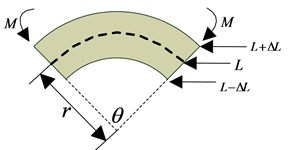
A length-preserving correspondence is established between deformed curved surface and original curved surface because there is a one-to-one correspondence of every point between after and before of the deformation, and the orthogonal relationship between two curves through nodes will not change under a micro deformation condition. So, the equal arc length grids mentioned above became an orthogonal curve net, as shown in Fig. 2.
Fig. 2Orthogonal curve net
If the coordinate of each node on orthogonal curve net showed in Fig. 2 can be solved separately by a certain computation method, the whole smooth curved surface can be obtained by traditional curved surface fitting algorithm. Considering that the research object is one-side fixed and there is no large deformation, there exist two boundary conditions:
1) There is no deformation on the fix side of curved surface,
2) The central line along direction of orthogonal curve net is plane curve.
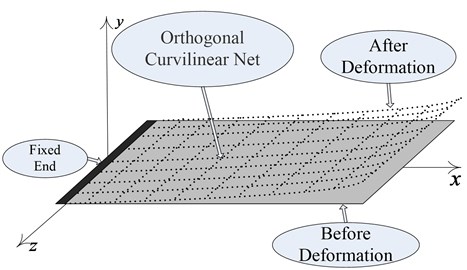
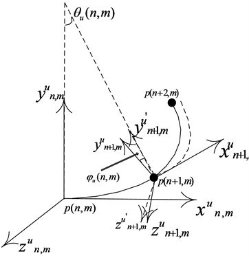
In order to describe the algorithm conveniently, the moving coordinate system is established along the direction and direction of orthogonal curve net separately as shown in Fig. 3.
To ensure the curve continuity, there is a coordinate transformation relationship between adjacent moving coordinate system on the curve. The relationship contains translation, rotation around axis and rotation around axis, as shown in Fig. 4.
In Fig. 4, , where is torsion angle. The transformation process is that moving the coordinate origin from point to point firstly. Then rotating degree around axis. Finally, rotating degree around axis. The torsion angle is obtained by the curvature coupling relationship between two orthogonal directions.
Fig. 3Moving coordinate system
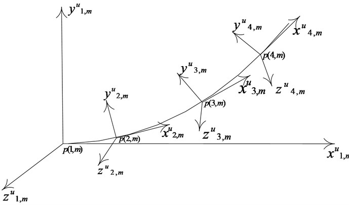
Fig. 4Moving coordinate system transformation
4.2. Nodal coordinate computation
The central line along direction is plane curve that can be obtained precisely by the curved fitting algorithm. Using the central line as the boundary, nodal coordinate of other curves can be obtained by iterative calculation. The micro arc between point and point is circle arc. , and is used to denote the coordinates of point separately. It is easy to know in the moving coordinate system that includes point , the coordinate of point is:
Assuming the point is the first point of the curve. The global coordinate system (absolute coordinate system) is established by using point as the original point. So, the absolute coordinate of point can be obtained by the following steps:
1) Rotate degree around axis.
2) Rotate degree around axis.
3) Move the original point from point to point .
So, if denotes the rotation transformation matrix that shows one point rotates degree around axis, the coordinate of point in absolute coordinate system is:
Similarly, the moving coordinate system where the point located has been transformed relative to absolute coordinate system as the following steps:
1) Rotate degree around axis.
2) Rotate degree around axis.
3) Move the original point from point to point .
4) Continue rotate degree around axis.
5) Continue rotate degree around axis.
6) Move the original point from point to point .
From the above transformation, the absolute coordinate of can be obtained:
The above formula can be simplified to:
And so on, the absolute coordinate (when ) of point can be obtained:
In Eq. (29), , is:
So far, one nodal coordinate can be computed according to Eq. (25) and Eqs. (29)-(31). All nodal coordinates can be obtained by iterative recursion combining with coupling transformation of the moving coordinate system.
Fig. 5Coupling relationship between orthogonal coordinate direction
4.3. Coupling transformation of the moving coordinate systems
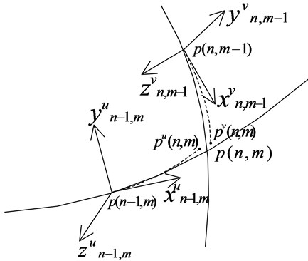
The moving coordinate systems along direction and along direction are moving along the curve on which they are located. And they converge on the next node of orthogonal curve net. On the basis of a nodal coordinate using to compute the coordinate of next node, coupling transformation between two moving coordinate system along two directions must be performed. If point and are the points in the moving coordinate system. The midpoint between points and is used as the valid value of node , as shown in Fig. 5. After the node is obtained, the moving coordinate system along direction and direction converge on the node . Because two curves at node are orthogonal, corresponding axes should converge. The torsion angle of two moving coordinate system can be obtained.
Firstly, axis and axis of the two coordinate systems rotate degree and degree around its own axis separately. and () are used to denote the obtained coordinate systems. The vector denotes axis of the moving coordinate system along direction, and so on. If is used to denote relative coordinate of vector in the coordinate system of , the torsion angles of the two moving coordinate system can be obtained:
The two coordinate systems should rotate degree around its axis separately to ensure superposition of corresponding coordinate axis:
Thus, new moving coordinate system along direction can be obtained:
In the same way, new moving coordinate system along direction can also be obtained:
In Eq. (34) and (35), the matrix of rotation angle around axis is:
Therefore, the coupling transformation of the two moving coordinate systems at the node can be obtained on the basis of Eq. (34) and Eq. (35). The coordinate of next node can be obtained based on the transformed moving coordinate system. All nodal coordinate on orthogonal curve net can be obtained by continuous iterative computation which contains node coordinate recursion and coupling transformation of moving coordinate system.
5. Experiment platform design and construction
5.1. Optimal placement of FBG sensors
While two kinds of structure shape reconstruction algorithm of experimental analysis and verification should be carried out under the same conditions. Two optimal placment configuration are designed with 25 pairs of FBG sensors. The constraint criterion for modal approach is shown as follows:
1) Space constraints. In order to avoid the repeated strain measurement information, the layout of the distance between every two points should have certain interval. The selection of the interval should be not less than 4 cm.
2) Reconstruction mean square error (MSE) constraints: denotes the displacement, represents the actual displacement, is the number of the surface point. Reconstruction mean square error can be defined as , which should be minimized.
The constraint criterion for the proposed approach is shown as follows:
1) Same rank constraints: Set the position of sensor measurement point as (. In order to carry out curvature data interpolation in the same row/column and convenient to carry out the curvature data interpolation, sensor measurement point should be in the same row or in the same column. Considering measuring points with columns, rank constraints is . In which is the sorted value of from small to large order.
2) Space constraints: As reconstruction algorithm is recursive, cumulative error is unavoidable in the iterative computation. To reduce the accumulation error effectively, the further the sensors located from the fixed end, the greater the space between the two sensors should be. So space constraints can be expressed as: , here:
3) Stress constraints: While the stress distribution of plate structure is , the sensor should be located in largest stress area. Set the maximum is , the minimum is , stress constraints is: .
The cost function can be obtained by weighted summing of the above constraints. Particle swarm optimization (PSO) algorithm is employed as the optimization algorithm. Each particle is corresponded to a solution of the problem. The information particle can be expressed with dimensional vector, the location is expressed as , speed is expressed as . The optimal location of the th particle is . The optimal location of a particle Historical optimal location of group is . Then the speed and position update equations is shown as follows:
Here, and is the random number between [0, 1], and is the acceleration coefficient, which is used to adjust the maximum step to the global optimal particle and the individual optimum particle. Usually, . is inertia weight, which controls the search area of the particles:
where, is the maximum value of inertia weight, is the minimum value of inertia weight. is the largest iteration number, is the current iteration number, reduce nonlinearly. The optimal placement of sensors for the modal approach and the proposed approach using PSO (Particle Swarm Optimization) is shown in Fig. 6 [20-22].
Fig. 6The optimal placement of sensors
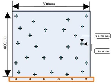
a) Optimization solutions for modal approach
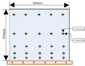
b) Optimization solutions for orthogonal curvilinear net method
5.2. Structural design of experiment model
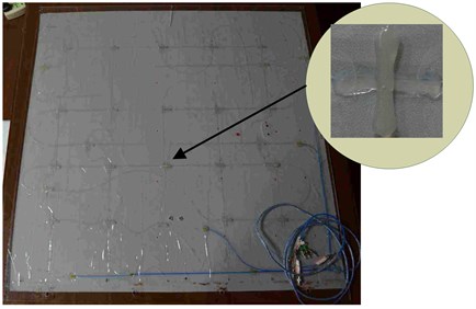
A square plexiglass plate was used as the experiment plate. The elastic modulus is 6.9×10⁹ Pa; Poisson’s ratio is ; the density is 1200 kg/m3; the size is 800×800×5 mm.The FBG sensors bonded on the sides of the plate orthogonally. Orthogonal FBG sensors can measure the structural strain in horizontal direction and vertical direction respectively at different measuring points. The signals are acquired by the FBG network analyzer. Considering the number constraints of grating point on the FBG network analyzer, the different optimization solutions for the two algorithm, we finally selected 32 pairs of FBG sensors to paste, and the layout scheme is shown as Fig. 7. The actual strain sensing network of FBG sensors is shown in Fig. 8.
Fig. 7Layout of FBG sensors
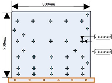
Fig. 8Smart plate structure with bonded FBG sensors
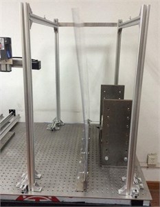
5.3. Experimental platform construction
With the constructed smart FBG plate, a vibration shape reconstruction experiment platform is built as shown in Fig. 8. The experimental platform contains a support base, the smart FBG plate, an excitation system, strain measurement system, displacement measurement system and shape reconstruction software system. The support base of the experiemental platform is an optical experiment table. The table type is GZ103PTB. The excitation system contains a signal generator, a power amplifier, and an exciter. The strain measurement system is consisted of the FBG sensors and the fiber grating network analyzer. It can collect the grating wavelength signal of the FBG sensors precisely for strain and curvature caculation. Displacement measurement system is consisted of three-dimensional guide, motion controller, motor driver, laser displacement sensor and data acquisition software. It can achieve real-time acquisition of the vibration displacement of the smart FBG plate. The software system contains a server and a client. The server is used for data transmission of the original data. The client is used for real time shape reconstruction. The reconstruction result can display dynamically and visually on the screen.
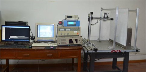
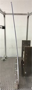
The photo of the experimental platform is shown in Fig. 9. The range of FBG sensor central wavelength is 1532 nm-1568 nm. The type of the fiber grating network analyzer is FONA-2008C. Its precision is 1 pm. The type of the signal generator is SFG-2110. The type of the power amplifier is YE5872. The type of the exciter is JZK-10 with maximum exciting force of 200 N. The model of laser displacement sensor is LK-GD500. The accuracy of the three dimensional guide is 0.0025 mm.
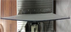
Fig. 9Schematic diagram of the experimental platform
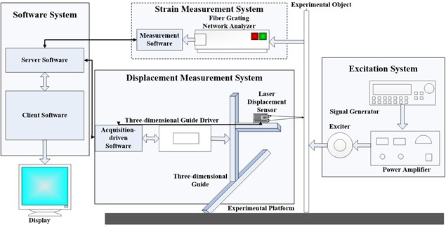
Fig. 10Photo of the experimental platform
In the experiment platform, the computer configuration is shown as follows:
• CPU: Intel(R) Core(TM)2 Quad CPU @2.50 GHz;
• RAM: Kingston DDR3 4 GB;
• Hard disk: Seagate ST2000VX000;
• Network adapter: Pealtec PCIe GBE Family Controller;
• GPU: NVIDIA GeForce 9600GS.
6. Experimental analysis and verification
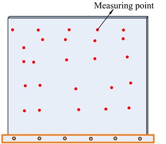
In order to evaluate the reconstruction effects and precision. 25 random measurement points were selected discretely on experiment model surface to analyze experimental precision of reconstruction for the static and dynamic deformation. The schematic diagram of selected measurement points is showed in Fig. 11.
Fig. 11Schematic diagram of selected measurement points
The reconstruction precision on one measuring point is defined in Eq. (40) to evaluate the practical effects of shape reconstruction algorithms quantitatively:
where, is the actual displacement on one measuring point (displacement measured by laser displacement sensor), and is the displacement reconstructed on that point:
where, is the number of measuring points. For the vibration shape reconstruction, the average accuracy of reconstruction on one measuring point is calculated by:
where, is the times of data acquisition on that measuring point.
6.1. Shape reconstruction for static deformation
Pure bending deformation and torsion deformation, were selected to reconstruct the shape of the plate structure. Firstly, make the experimental model to produce pure bending deformation that the largest range of deflection on the free end was less than ±10 cm, and reconstruct the shape with the two different algorithms respectively. The experimental data on 8 different kinds of deformation were measured and reconstructed to verify and compare the algorithms. The average accuracies of reconstruction were calculated according the Eq. (38), and the experimental results were shown in Table 1.
As can be seen from Table 1, for the pure bending deformation, the two reconstruction algorithms both have high accuracy. When the deformation is small, the reconstruction accuracy of modal approach is higher than orthogonal curvilinear net method. With the increase of deformation, the reconstruction accuracy of the orthogonal curvilinear net method gradually increases, and in the large deformation, the reconstruction effect is better than that of displacement reconstructed by modal approach, which shows that the orthogonal curvilinear net method is more suitable for large static pure bending deformation of shape reconstruction, and the modal approach is more suitable for small deformation.
Adopting the same experimental verification and data analysis method, make the experimental model to produce torsion deformation that the largest deflection on the free end was less than ±5 cm, and select 4 different kinds of deformation to reconstruct and compare with the two algorithms. The experimental results were shown in Table 2.
Table 1The experimental results of pure bending deformation
Algorithms | Deformations | |||||||
–10 cm | –8 cm | –5 cm | –2 cm | 2 cm | 5 cm | 8 cm | 10 cm | |
Modal approach | 90.32 % | 90.41 % | 90.95 % | 89.76 % | 90.79 % | 91.85 % | 91.07 % | 90.09 % |
Orthogonal curvilinear net method | 95.39 % | 90.45 % | 90.65 % | 81.15 % | 85.07 % | 89.40 % | 93.34 % | 95.69 % |
Table 2The experimental results of torsion deformation
Algorithms | Deformations | |||
–5 cm | –2 cm | 2 cm | 5 cm | |
Modal approach | 84.64 % | 86.27 % | 85.38 % | 83.39 % |
Orthogonal curvilinear net method | 92.23 % | 82.49 % | 81.47 % | 89.49 % |
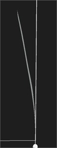
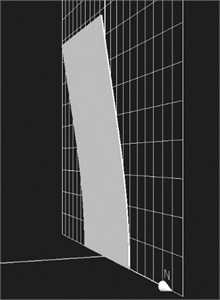
The analytic results of reconstruction accuracy presented in Table 2 are basically consistent with the results shown in Table 1. For the static torsion deformation, the deformation amount is small, and the reconstruction effect of modal approach is better than the orthogonal curvilinear net method; when the deformation amount enlarge, the orthogonal curvilinear net method is better than modal approach. The reconstruction effects of static experiment are shown in Fig. 12.
Fig. 12Reconstruction performance for static deformation
a) Pure bending deformation
b) Shape reconstructed by modal approach
c) Shape reconstructed by orthogonal curvilinear net method
d) Torsion deformation

e) Shape reconstructed by modal approach

f) Shape reconstructed by orthogonal curvilinear net method
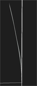
The actual pure bending deformation is shown in Fig. 12(a), and the shape reconstruction effects by modal approach and orthogonal curvilinear net method are shown in Fig. 12(b) and Fig. 12(c). Moreover, the actual torsion deformation is shown in Fig. 12(d), and the shape reconstruction effects by modal approach and orthogonal curvilinear net method are shown in Fig. 12(e) and Fig. 12(f). As shown in Fig. 12, the shape reconstruction results of two algorithms have good visual effects for pure bending deformation and torsion deformation, which demonstrate that the effectiveness and feasibility of the both algorithms.
6.2. Dynamic vibration shape reconstruction
The first-order natural frequency of the smart plate is 2.3 Hz, the second-order natural frequency is 4.2 Hz, the third-order natural frequency is 5.9 Hz. Fig. 13 illustrates the recontruction performance at the second-order natural frequency.
Fig. 13Reconstruction performance for dynamic vibration at the second-order natural frequency
a) Dynamic vibration shape
b) Shape reconstructed by modal approach
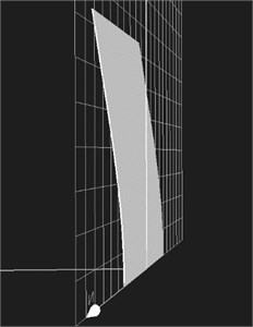
c) Shape reconstructed by orthogonal curvilinear net method
The reconstruction accuracy on each measuring point was calculated by Eq. (39), and the experiment results are shown in Fig. 14.
Fig. 14Experimental results for dynamic vibration shape reconstruction
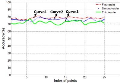
a) Experimental results of modal approach
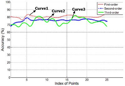
b) Experimental results of orthogonal curvilinear net method
In Fig. 14, axis represents the serial number of the measuring point, a total of 25 points, and the y axis represents accuracy. Fig. 14(a) is the experimental results of modal approach, and Fig. 14(b) is the experimental results of orthogonal curve net method. From Fig. 14 we can draw the following conclusions:
• For the first-order natural frequency, the reconstruction accuracy of orthogonal curvilinear net method is higher than modal approach.
• With the increase of the vibration frequency, reconstruction accuracy of the two algorithms decrease.
• Under the high-order natural frequency, reconstruction accuracy of modal approach is more balanced than orthogonal curvilinear net method.
In short, orthogonal curvilinear net method is more suitable for low frequency vibration, modal approach is more applicable to high frequency of vibration. For a clearer understanding of the difference between the reconstructed displacement and the actual displacement of a point, comparison of the reconstructed displacement and actual displacement on the fifth point is shown in Fig. 15.
Fig. 15Comparison of the reconstructed displacement and actual displacement
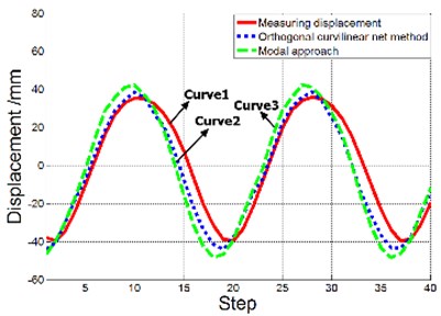
a) First natural frequency
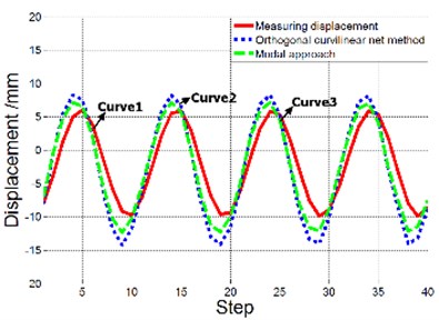
b) Second natural frequency
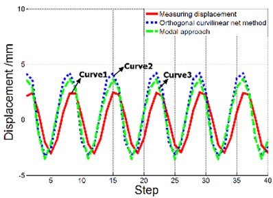
c) Third natural frequency
6.3. Algorithm efficiency analysis
To analyze the operation efficiency of the algorithms, the time consumption on different types of experiments of the two algorithms was counted, and the statistical results were shown in Table 3.
Table 3Time consumption of processing a frame of data
Algorithm | Experiment type | ||
Pure bending deformation | Torsion deformation | Dynamic vibration | |
Modal approach | 23.516 ms | 24.247 ms | 24.031 ms |
Orthogonal curvilinear net method | 20.341 ms | 20.919 ms | 20.377 ms |
In Table 3, for different experiment types, there was no obvious difference on the time consumption. While the time consumption of orthogonal curvilinear net method was lower than the modal approach, showing that the orthogonal curvilinear net method is superior than modal approach in computational efficiency.
6.4. Sensitivity analysis
When the FBG sensor is used as strain sensor, the resolution of strain measurement is 1 με. 10 με could be considered as a reliable value for shape reconstruction. While each sensor is subjected to the same 10 με strain in the same direction. The curved deformation of the plate structure is shown in Fig. 16.
Fig. 16Curved deformation of the plate structure
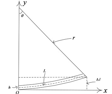
is the central angle for the bending plate structure. is the radius of the circular arc. is the arc length of the neutral surface. 800 mm. is the thickness of the structure model, 5 mm. is the free end displacement, and it is theoretical sensitivity. The following relationship could be established:
Thus, the theoretical sensitivity of the proposed structural reconstruction algorithm is 0.00039 mm. But in the experiment process, considering the strain-curvature conversion error, the interpolation calculation error, and the approximate calculation of the coordinate system torsional angle, the experimental sensitivity should be greater than 0.00039 mm. But unfortunately the experimental setup could not give so small deformation.
7. Conclusions
On the basis of analyzing the principle of the FBG sensors and its configuration method, we have studied curved surface reconstruction algorithm based on the modal approach, and proposed a new curved surface reconstruction algorithm based on orthogonal curvilinear net. The process of iterative computing is deduced. A high precision experiment platform is built. Reconstruction accuracies and performance of both algorithms are analyzed. The experimental results show: the reconstruction effect of the orthogonal curvilinear net method is better than modal approach for large static deformation or large low frequency vibration. However, for small static deformation or relatively high frequency vibration, the reconstruction effect of displacement by modal approach is better than orthogonal curvilinear net method. Moreover, the computing efficiency of orthogonal curvilinear net method is superior to the modal approach. Therefore, for large deformation, low frequency or strict real-time applications, orthogonal curvilinear net method will be a suitable method. Otherwise, the modal approach may be a good choice.
References
-
Voland R. T., Huebner L. D., McClinton C. R. X-43a hypersonic vehicle technology development. Acta Astronautica, Vol. 59, Issue 1, 2006, p. 181-191.
-
Weinzettel J., Reenaas M., Solli C., Hertwich E. G. Life cycle assessment of a floating offshore wind turbine. Renewable Energy, Vol. 34, Issue 3, 2009, p. 742-747.
-
Derkevorkian A., Masri S. F., Alvarenga J., Boussalis H., Bakalyar J., Richards W. L. Strain-based deformation shape-estimation algorithm for control and monitoring applications. AIAA Journal, Vol. 51, Issue 9, 2013, p. 2231-2240.
-
Minakuchi S., Takeda N. Recent advancement in optical fiber sensing for aerospace composite structures. Photonic Sensors, Vol. 3, Issue 4, 2013, p. 345-354.
-
Liu T., Burner A. W., Jones T. W., Barrows D. A. Photogrammetric techniques for aerospace applications. Progress in Aerospace Sciences, Vol. 54, 2012, p. 1-58.
-
Qiu Z.-C., Zhang X.-T., Zhang X.-M. A vision-based vibration sensing and active control for a piezoelectric flexible cantilever plate. Journal of Vibration and Control, 2014.
-
Kiang C. T., Spowage A., Yoong C. K. Review of control and sensor system of flexible manipulator. Journal of Intelligent and Robotic Systems, Vol. 77, Issue 1, 2015, p. 187-213.
-
Park S., Park H., Kim J., Adeli H. 3D displacement measurement model for health monitoring of structures using a motion capture system. Measurement, Vol. 59, 2015, p. 352-362.
-
Panopoulou A., Loutas T., Roulias D., Fransen S., Kostopoulos V. Dynamic fiber Bragg gratings based health monitoring system of composite aerospace structures. Acta Astronautics, Vol. 69, Issue 7, 2011, p. 445-457.
-
Li W., Cheng C., Lo Y. Investigation of strain transmission of surface-bonded Fbgs used as strain sensors. Sensors and Actuators A: Physical, Vol. 149, Issue 2, 2009, p. 201-207.
-
Payo I., Feliu V., Cortázar O. D. Fibre Bragg grating (Fbg) sensor system for highly flexible single-link robots. Sensors and Actuators A: Physical, Vol. 150, Issue 1, 2009, p. 24-39.
-
Mieloszyk M., Skarbek L., Krawczuk M., Ostachowicz W., Zak A. Application of fibre Bragg grating sensors for structural health monitoring of an adaptive wing. Smart Materials and Structures, Vol. 20, Issue 12, 2011, p. 125014.
-
Bang H.-J., Ko S.-W., Jang M.-S., Kim H.-I. Shape estimation and health monitoring of wind turbine tower using an Fbg sensor array. IEEE International on Instrumentation and Measurement Technology Conference (I2MTC), 2012, p. 496-500.
-
Ling H.-Y., Lau K.-T., Cheng L., Jin W. Viability of using an embedded Fbg sensor in a composite structure for dynamic strain measurement. Measurement, Vol. 39, Issue 4, 2006, p. 328-334.
-
Kang L.-H., Kim D.-K., Han J.-H. Estimation of dynamic structural displacements using fiber Bragg grating strain sensors. Journal of Sound and Vibration, Vol. 305, Issue 3, 2007, p. 534-542.
-
Rapp S., Kang L.-H., Han J.-H., Mueller U. C., Baier H. Displacement field estimation for a two-dimensional structure using fiber bragg grating sensors. Smart Materials and Structures, Vol. 18, Issue 2, 2009, p. 025006.
-
Yi J., Zhu X., Zhang H., Shen L., Qiao X. Spatial Shape reconstruction using orthogonal fiber bragg grating sensor array. Mechatronics, Vol. 22, Issue 6, 2012, p. 679-687.
-
Li L., Li W., Ding P., Zhu X., Sun W. Structural shape reconstruction through modal approach using strain gages. Computational Intelligence, Networked Systems and Their Applications, Vol. 462, 2014, p. 283-281
-
Wang Y., Zheng J. Curvature-guided adaptive T-spline surface fitting. Computer-Aided Design, Vol. 45, Issue 8, 2013, p. 1095-1107.
-
Di H. Space curve fitting method based on fiber-optic curvature gages. Optics and Laser Technology, Vol. 44, Issue 1, 2012, p. 290-294.
About this article

This paper is sponsored by program of National Natural Science Foundation of China (No. 51175319), Innovation program of Shanghai Municipal Education Commission (No. 13ZZ075), and Shanghai Key Laboratory of Power Station Automation Technology.
