Dynamics analysis for the clamping mechanisms of a rotary inchworm piezoelectric motor

Gu, Yongfei; Xing, Jichun

doi:10.21595/jve.2016.16005

Journal of Vibroengineering

Browse Journal

Submit article

Published: 30 June 2016

Check for updates

Dynamics analysis for the clamping mechanisms of a rotary inchworm piezoelectric motor

Yongfei Gu¹

Jichun Xing²

¹Education Ministry Key Laboratory of Advanced Forging and Stamping Technology and Science, Yanshan University, Qinhuangdao, China

^{1, 2}School of Mechanical Engineering, Yanshan University, Qinhuangdao, China

Corresponding Author:

Jichun Xing

Cite the article Download PDF

Downloads 1546

WoS Core Citations 4

CrossRef Citations 3

Abstract

In this study, a rotary inchworm piezoelectric motor is proposed. The operating principle of the proposed motor and its clamping mechanisms are discussed. Moreover, we also establish the dynamic equation of the clamping mechanisms. From the established equations, the natural frequencies and modal functions are obtained. The sensitivities of the configuration parameter to natural frequencies of the clamping mechanisms are investigated. Finally, the tests on the relative errors of the natural frequencies between the theoretical and experimented results are performed to verity the correctness of the theoretical analysis.

1. Introduction

Piezoelectric motors, which can be classified by their operation frequency, are used for micro/macro positioning in the longitudinal and rotary directions [1]. Quasi-static motors, such as inchworm piezoelectric motors and inertial impact motors, were operated at low frequency with a stable response. Ultrasonic motors were operated at a high frequency, in which traveling wave ultrasonic motors have been carried out the topic of a large number of studies on and achieved prominent results [2, 3]. The most common type of rotary piezoelectric motors is the traveling wave ultrasonic motor. Its rotational speed is high but the positioning accuracy and resolution under high-precision positioning is low [4]. By contrast, inchworm piezoelectric motors feature a large stroke with high accuracy and resolution. This type of motors can also overcome the output torque shortage of inertial impact piezoelectric motors [5].

As an important type of piezoelectric motors, inchworm piezoelectric motors have been successfully applied in precision driving [6]. However, most existing inchworm piezoelectric motors are used for positioning in the longitudinal direction. The principle of inchworm motion is rarely applied in precision rotational driving field. Therefore, the application of inchworm piezoelectric motors in precision control are limited [7].

The present study proposes a novel type of rotary inchworm piezoelectric precision motor. A dynamic model of clamping mechanisms (CMs) is also put forward. The natural frequencies and modal functions are obtained. And the effects of the principal factors that influence the natural frequencies are investigated. A prototype motor is finally developed. The experimental results of the natural frequency of the clamping mechanisms are consistent with the theoretical analysis.

2. Motor description

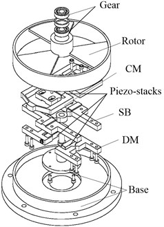
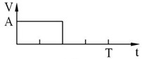
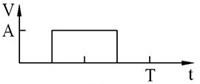
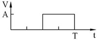
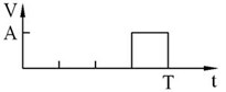
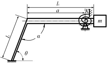
The motor consists of a stator and a rotor (see Fig. 1). The stator consists of two CMs, two driving mechanisms (DMs), and a swinger base (SB). The two CMs are symmetrically mounted on an upper SB to grip the rotor alternately. The two DMs are symmetrically mounted on a lower SB to create an angular displacement. A square wave voltage signal at a special frequency is input to four piezo-stacks to make the motor move (see Fig. 2 for the sequence of voltage signals in a cycle). The operating principle of the motor is shown in Fig. 2.

Fig. 1Rotary inchworm piezoelectric motor

The working procedure of the motor is as follows:

1. The contact shoe of CM(A) is extended and clamped onto the rotor.

2. As DM(A) is bent by piezo-stack(B), the arm of SB rotates at an angle $θ$ .

3. The contact shoe of CM(A)contracts and releases the rotor, while the contact shoe of CM(B) is extended and clamped onto the rotor. The rotor remains stationary during the process.

4. The arm of SB is restored to the original state, and the rotor is again rotated at an angle $θ$ .

5. As the DM(B) is bent by piezo-stack (D), the arm of SB is rotated at an angle $θ$ again. The contact shoe of CM(B)contracts and releases the rotor and the arm of SB is restored to its original state. The steps 1 to 5 are repeated to achieve continuous working of the motor

Fig. 2Driving principal schematic

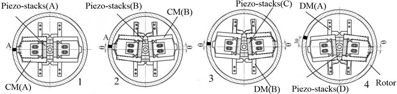
Fig. 3Driving signal

3. Dynamics model of the clamping mechanisms

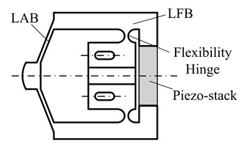
Each CM which is driven by the piezo-stack integrates lever and triangle amplification to achieve contact shoe displacement amplification. The configuration of CMs is shown in Fig. 4. When the motor is operated, the deformation of the CMs mainly occurred in the lever amplification beam (LAB) and the long flexibility beam (LFB). The symmetric vibration modes of the CMs are considered, because of their symmetric structure. The dynamic of half a CM is analyzed. The simplified dynamic model is based on the following assumptions:

Fig. 4Displacement amplification principle

1) The ratio of LAB thickness to its length is more than 0.2. Given the impact of cross-section rotational inertia, the LAB is a Timoshenko beam.

2) The boundary condition on the right end of the LAB is considered as lumped mass $m$ .

3) The bending deformation of flexible hinge is considered, while tensile deformation is ignored. Hence, the flexible hinge is considered both as a hinge and as a coil spring. The rotational stiffness equation for a straight round flexible hinge, which is deduced by Yingfei Wu and Zhaoying Zhou [8], is as follows:

1

K = \frac{E b R^{2}}{12 f_{2}},

2

f_{2} = \frac{2 s^{3} (6 s^{2} + 4 s + 1)}{(2 s + 1) {(4 s + 1)}^{2}} + \frac{12 s^{4} (2 s + 1)}{{(4 s + 1)}^{\frac{5}{2}}} a r c t a n \sqrt{4 s + 1},

3

s = \frac{R}{t},

where $E$ is the modulus of elasticity of the material for the CMs, $b$ is the width of the flexible hinge, $t$ is the thickness of the recess of flexible hinge, and $R$ is the notch radius of the flexible hinge.

4) The boundary condition on the right end of the LAB is considered as a fixed end.

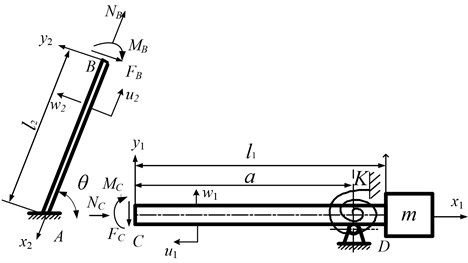
5) Considering the bending and longitudinal vibration deformations of the LAB and LFB, the dynamic model of the CMs is simplified into two uniform beams. Fig. 5 describes the two uniform beams, where the $x$ -axis is along the $x_{i}$ ( $i =$ 1, 2), the $y$ -axis is along the $y_{i}$ , and the origin is B(C).

Fig. 5Dynamic model of the CMs

3.1. The longitudinal vibration of beams

Suppose the cross section of the beam in the model remains a plane in the vibration process. The dynamic equation of the beam in the longitudinal vibration is as follows:

4

\frac{\partial^{2} u_{i} (x_{i}, t)}{\partial t^{2}} = \frac{E}{ρ} \frac{\partial^{2} u_{i} (x_{i}, t)}{\partial x_{i}^{2}},

where $u_{i} (x_{i}, t)$ is the displacement of the beam longitudinal direction, $x_{i}$ is the length coordinate of the beam, $t$ is thetime, $ρ$ is the material density of the CMs, and $E$ is the elasticity modulus of the CMs material.

Let $u_{i} (x_{i}, t) = φ_{u i} (x_{i}) q (t)$ . Then, the longitudinal vibration mode function of the beam is:

5

φ_{u_{i}} (x) = {D_{1}}_{i} c o s β x_{i} + {D_{2}}_{i} s i n β x_{i},

where $β^{2} = ρ ω^{2} / E$ .

3.2. Bending vibration of LAB

Consider the LAB as a Timoshenko beam, the dynamic equation of the bending vibration of LAB can be given as follows:

6

\frac{\partial^{2} w_{1}}{\partial t^{2}} + \frac{E I_{1}}{ρ S_{1}} \frac{\partial^{4} w_{1}}{\partial x_{1}^{4}} - \frac{I_{1}}{S_{1}} (1 + \frac{E}{κ G}) \frac{\partial^{4} w_{1}}{\partial x_{1}^{2} \partial t^{2}} + \frac{ρ I_{1}}{S_{1} κ G} \frac{\partial^{4} w_{1}}{\partial t^{2}} = 0,

where $w_{1} (x_{1}, t)$ is the transverse displacement of the beam, $κ$ is the section factor, $G$ is the shear modulus, $I_{1}$ is the second moment of the area of the LAB, and $S_{1}$ is the section area of the LAB. The effect of section moment of inertia is considered, while shear deformation is ignored. Thus, we obtain:

7

\frac{\partial^{2} w_{1}}{\partial t^{2}} + \frac{E I_{1}}{ρ S_{1}} \frac{\partial^{4} w_{1}}{\partial x_{1}^{4}} - \frac{I_{1}}{S_{1}} \frac{\partial^{4} w_{1}}{\partial x_{1}^{2} \partial t^{2}} = 0 .

Let $w_{1} (x_{1}, t) = φ_{w 1} (x_{1}) q (t)$ . The bending vibration mode function of the LAB can then be shown as:

8

φ_{w 1} (x) = C_{1} c o s s_{1} x_{1} + C_{2} s i n s_{1} x_{1} + C_{3} c o s h s_{2} x_{1} + C_{4} s i n h s_{2} x_{1},

where:

s_{1} = \sqrt{\sqrt{γ^{4} + \frac{δ^{4}}{4}} + \frac{δ^{2}}{2}}, s_{2} = \sqrt{\sqrt{γ^{4} + \frac{δ^{4}}{4}} - \frac{δ^{2}}{2}}, γ^{4} = \frac{ρ S_{1} ω^{2}}{E I_{1}}, δ^{2} = \frac{ρ ω^{2}}{E} .

3.3. Bending vibration of LFB

The LFB is described as a Euler Bernoulli beam, and its axial deformation and transverse deformation in the $z$ direction are assumed to be negligible. The dynamic equations of the LFB is:

9

\frac{\partial^{2}}{\partial {x_{2}}^{2}} [E I_{2} (x_{2}) \frac{\partial^{2} w_{2} (x_{2}, t)}{\partial x_{2}^{2}}] + ρ S_{2} (x_{2}) \frac{\partial^{2} w_{2} (x_{2}, t)}{\partial t^{2}} = 0,

where $S_{2} (x_{2})$ is the area of section, and $I_{2} (x)$ is the second moment of the area of the LFB. Let $w_{2} (x_{2}, t) = φ_{w 2} (x_{2}) q (t)$ . The bending vibration mode function of the LFB is:

10

φ_{w 2} (x) = B_{1} c o s p x_{2} + B_{2} s i n p x_{2} + B_{3} c o s h p x_{2} + B_{4} s i n h p x_{2},

where $p^{4} = ρ S^{2} ω^{2} / E I^{2}$ .

3.4. Boundary conditions

When are end of LFB (end A) is fixed, its boundary conditions are as follows:

11

\{\begin{array}{l} φ_{w_{2}} (l_{2}) = 0, \\ {φ'}_{w_{2}} (l_{2}) = 0, \\ φ_{u 2} (l_{2}) = 0 . \end{array}

The distance between the hinge and the origin is approximately equal to the length of the LAB ( $a \approx l_{1}$ ), because mass $m$ is near the hinge. Thus, the boundary conditions of the end D of the LAB is:

12

\{\begin{array}{l} φ_{w 1} (l_{1}) = 0, \\ E I φ_{w 1}^{''} (l_{1}) = - K φ_{w 1}^{'} (l_{1}), \\ φ_{u 1} (l_{1}) = 0 . \end{array}

Considering the longitudinal and bending vibration at the junction of two beams, we obtain the displacement relationship between point B and C:

13

\{\begin{array}{l} u_{2} s i n θ + w_{2} c o s θ = w_{1}, \\ w_{2} s i n θ - u_{2} c o s θ = u_{1}, \\ ζ_{B} = ζ_{C}, \end{array}

where $ζ_{B}$ is the rotation angle of point B, and $ζ_{C}$ is the rotation angle of point C. Based on continuity conditions, the equilibrium conditions of the generalized force of the point B and C can be obtained as:

14

\{\begin{array}{l} M_{B} + M_{C} = 0, \\ N_{B} c o s θ + F_{B} s i n θ + N_{C} = 0, \\ N_{B} s i n θ + F_{B} c o s θ - F_{C} = 0, \end{array}

where $M_{B (C)}$ is the bending moment of point B(C), $F_{B (C)}$ is the shearing force of point B(C), and $N_{B (C)}$ is the pulling force of point B(C). Substitute the boundary conditions Eq. (11) to Eq. (14), Eqs. (6), (8), and Eq. (10) yields:

15

\{\begin{array}{l} B_{1} c o s p l_{2} + B_{2} s i n p l_{2} + B_{3} c o s h p l_{2} + B_{4} s i n h p l_{2} = 0, \\ - B_{1} s i n p l_{2} + B_{2} c o s p l_{2} + B_{3} s i n h p l_{2} + B_{4} c o s h p l_{2} = 0, \\ D_{21} c o s β l_{2} + D_{22} s i n β l_{2} = 0, \\ C_{1} c o s s_{1} a + C_{2} s i n s_{1} a + C_{3} c o s h s_{2} a + C_{4} s i n h s_{2} a = 0, \\ (\begin{array}{l} - C_{1} s_{1}^{2} c o s s_{1} a - C_{2} s_{1}^{2} s i n s_{1} a + C_{3} s_{2}^{2} c o s h s_{2} a + C_{4} s_{2}^{2} s i n h s_{2} a \\ = - \frac{K}{E I_{1}} (- C_{1} s_{1} s i n s_{1} a + C_{2} s_{1} c o s s_{1} a + C_{3} s_{2} s i n h s_{2} a + C_{4} s_{2} c o s h s_{2} a) \end{array}), \\ D_{11} c o s β a + D_{12} s i n β a = 0, \\ B_{1} c o s θ + B_{3} c o s θ - C_{1} - C_{3} + D_{21} s i n θ = 0, \\ B_{1} s i n θ + B_{3} s i n θ - D_{11} - D_{21} c o s θ = 0, \\ I_{2} p B_{2} + I_{2} p B_{4} - I_{1} s_{1} C_{2} - I_{1} s_{2} C_{4} = 0, \\ - I_{2} p^{2} B_{1} + I_{2} p^{2} B_{3} - I_{1} s_{1}^{2} C_{1} + I_{1} s_{2}^{2} C_{3} = 0, \\ - I_{2} p^{3} s i n θ B_{2} + I_{2} p^{3} s i n θ B_{4} + A_{1} β D_{12} + A_{2} β c o s θ D_{22} = 0, \\ - I_{2} p^{3} c o s θ B_{2} + I_{2} p^{3} c o s θ B_{4} + I_{1} s_{1}^{3} C_{2} - I_{1} s_{2}^{3} C_{4} + A_{2} β s i n θ D_{22} = 0, \end{array}

where $l_{1}$ is the length of the LAB, $l_{2}$ is the length of the LFB, $θ$ is the angle between the LFB and the horizontal direction. The coefficients $D_{1 i}$ ( $i =$ 1, 2), $D_{2 i}$ , $C_{j}$ ( $j =$ 1, 2, 3, 4), $B_{j}$ , and $ω$ can be obtained through substitute of the boundary conditions.

4. Results and discussions

4.1. Natural frequency and mode function

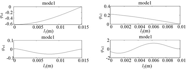
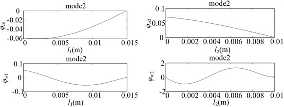
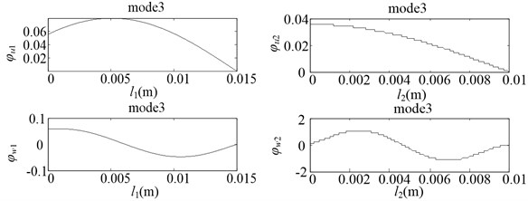
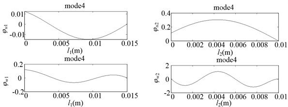
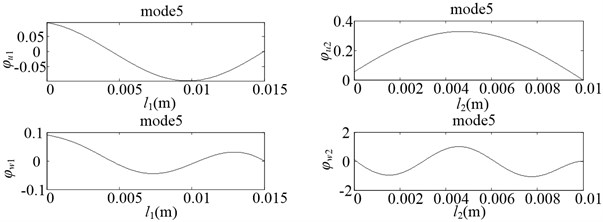
The Eq. (15) is utilized in the free vibration analysis of the CMs to obtain the natural frequencies and vibration modes. The configuration parameters of the CMs are shown in Table 1. The material of the CMs is brass. Table 2 lists the first eight natural frequencies of the CMs. The vibration modes of the CMs are shown in Fig. 7. From Table 2 and Fig. 7, the following observations are worth noting.

1) In the first eight natural frequencies, the natural frequency of mode 3 and mode 4 is close, the difference is 333 Hz; The natural frequency of mode 6 and mode 7 is close, the difference is 109 Hz.

2) In the first five vibration modes, the longitudinal vibration of two beams (LAB and LFB) exist one peak. As the orders of the vibration modes increases, the position of the peak moves from the origin to the $x_{1} (x_{2})$ direction. In mode 1 and mode 3, the maximum deformation of the longitudinal vibration of the LAB is greater than that of the LFB.

Fig. 7Vibration modes of the CMs

a)

b)

c)

d)

e)

3) The LAB has greater thickness than the LFB. Thus, the number of peaks of the LAB is less than that of the LFB in the same order of vibration mode. The maximum deformation of the bending vibration of the LAB is also less than that of the LFB.

Table 1Parameters of the clamping mechanism

$ρ$ (kg/m³)	$E$ (GPa)	$b$ (mm)	$t$ (mm)	$h$ (mm)	$l_{1}$ (mm)	$h_{1}$ (mm)	$l_{2}$ (mm)	$h_{2}$ (mm)	$θ$
8900	90	5	1	5	10	1	15	5	70°

Table 2Natural frequency (Hz)

$ω_{1}$	$ω_{2}$	$ω_{3}$	$ω_{4}$	$ω_{5}$	$ω_{6}$	$ω_{7}$	$ω_{8}$
1704	1948	2535	4435	4768	5431	5540	7900

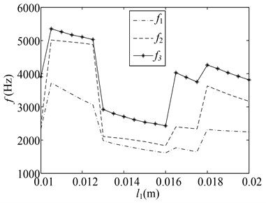
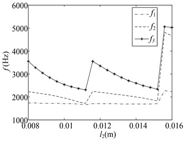
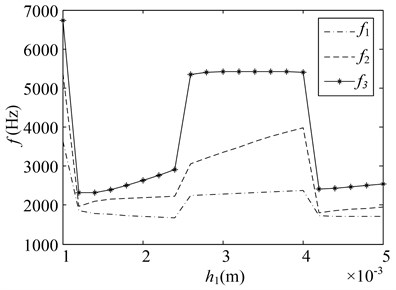
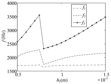
Fig. 8Changes of natural frequencies with respect to various parameters

a) $θ$ change

b) $l_{1}$ change

c) $l_{2}$ change

d) $h_{1}$ change

e) $h_{2}$ change

f) $t$ change

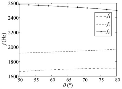
4.2. Sensibility analysis

We investigate the changes of CMs natural frequency along with the configuration parameters. The changes of natural frequency are shown in Fig. 8. The materials of the CMs and corresponding first three natural frequencies are shown in Table 3.

Table 3The first three natural frequency of different material

Material	Modulus of elasticity $E$ (N/m²)	Density $ρ$ (kg/m³)	Frequency
Material	Modulus of elasticity $E$ (N/m²)	Density $ρ$ (kg/m³)	$ω_{1}$ (Hz)	$ω_{2}$ (Hz)	$ω_{3}$ (Hz)
Aluminum	65×10⁹	2.7×10³	2629	3005	3912
Carbon steel	206×10⁹	7.7×10³	2771	3168	4124
Brass	90×10⁹	8.9×10³	1704	1947	2535
Alloy steel	206×10⁹	7.9×10³	2736	3127	4071
Gray pig iron	120×10⁹	7×10³	2218	2535	3301

The following observations are drawn:

1) As the horizontal angle of the LFB changes between 50° and 80°, the first-order and second-order natural frequency grows nonlinear, while the third natural frequency drops nonlinear.

2) When the length and thickness of the LAB and LFB change, the change in the natural frequency is irregularly serrate. In the change interval for some parameters ( $l_{1}$ , $h_{1}$ , $l_{2}$ , $h_{2}$ ), the natural frequency drops as the length of the LAB and LFB increases, the natural frequency drops; With the increase of the thickness of the LAB and the LFB, the natural frequency nonlinearity increases. When the parameters ( $l_{1}$ , $h_{1}$ , $l_{2}$ , $h_{2}$ ) change to a certain value, (e.g., $l_{1} =$ 10.5, 12.5, 16.5, 18 mm, $l_{2} =$ 11.6, 15.6 mm, $h_{1} =$ 1.2, 2.6, 4, $h_{2} =$ 0.8 mm), the curve of the natural frequency changes and mutates. This phenomenon can be attributed to the mutation of the vibration modes of the CMs under these parameters values.

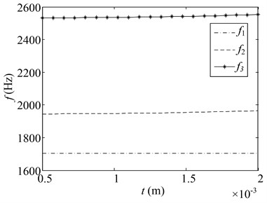
3) When the notch thickness of the flexible hinge changes between 0.5 and 2 mm, the natural frequency of the CMs slowly increases. The growth trend of the natural frequency becomes significant as the order number increases.

4) The natural frequency of each order is lower when brass is used as CMs material than when other materials are used. By contrast, the natural frequency of each order is higher when carbon steel is used as CMs material than when other materials are used.

5. TEST

The natural frequencies of the CMs are obtained by using the SZCJ knocking vibration tests system (see Fig. 9). The experimental results are shown in Fig. 10.

Fig. 9Impact hammer modal test

The relative errors are obtained by comparing the theoretical values and the experimental results. Table 4 shows that the relative errors in the first three natural frequencies are 2.7 %, 2.7 %, and 2.6 %. These relative errors are less than 3.0 % suggesting the reasonable agreement of the experimental results with the results of our theoretical analysis.

Table 4Comparison of experimental results and theoretical values

Frequency	$ω_{1}$ (Hz)	$ω_{2}$ (Hz)	$ω_{3}$ (Hz)
Theoretical values	1704	1948	2535
Experimental results	1751.7	2002.5	2602.5
Relative errors	2.7 %	2.7 %	2.6 %

Fig. 10Experimental results (Sample frequency = 10000.00 Hz)

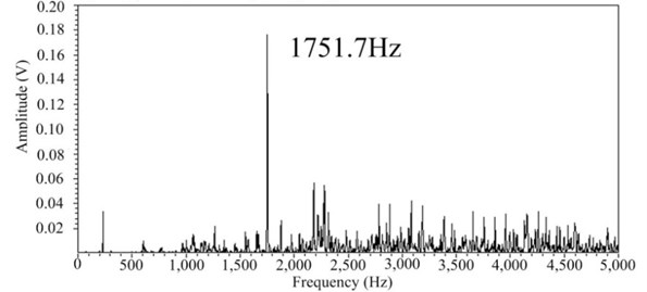
a) Mode 1

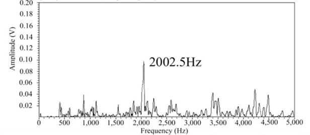
b) Mode 2

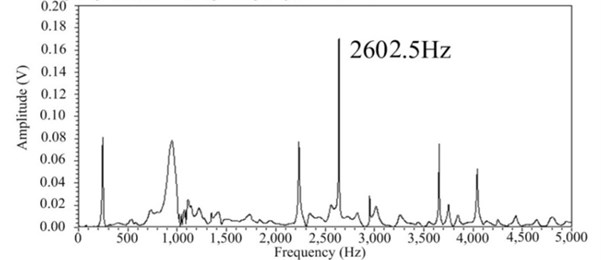
c) Mode 3

6. Conclusions

A novel rotary inchworm piezoelectric motor was proposed and the drive principle was discussed. The dynamic equations of the CMs were established. The natural frequencies and vibration modes were obtained, and the sensibility of the CMs was investigated. The relative errors of the natural frequency between the theoretical and experimental results verify the correctness of the theoretical analysis. This dynamic analysis of the CMs lays a theoretical foundation for the design of a novel rotary inchworm piezoelectric motor.

References

Duong Khanh, Garcia Ephrahim Design and performance of a rotary motor driven by piezoelectric stack actuators. Japanese Journal of Applied Physics, Vol. 35, Issue 12, 1996, p. 6334-6341.

Publisher
Vaughan Mark, Leo Donald J. Integrated piezoelectric linear motor for vehicle applications. ASME International Adaptive Structures and Materials Systems Symposium, New Orleans, 2002, p. 1-9.

Publisher
Cusin P., Sawai T., Konishi S. Compact and precise positioner based on the inchworm principle. Journal of Micromechanics and Microengineering, Vol. 10, Issue 4, 2000, p. 516-521.

Publisher
Duong Khanh, Garcia Ephrahim Development of a rotary inchworm piezoelectric motor. Smart Structures and Materials: Smart Structures and Integrated Systems, Vol. 2443, 1995, p. 752-788.

Publisher
Morita T., Murakami H., Yokose T., Hosaka H. A miniaturized resonant-type smooth impact drives mechanism actuator. Sensors and Actuators A, Vol. 178, 2012, p. 188-192.

Publisher
Tenzer P. E., Ben M. R. A systematic procedure for the design of piezoelectric inchworm precision position. IEEE/ASME Transactions on Mechatronics, Vol. 9, Issue 2, 2004, p. 427-435.

Publisher
Li J., Ramin S., Javad D. Design and development of a new piezoelectric linear inchworm actuator. Mechatronics, Vol. 15, 2005, p. 651-681.

Publisher
Wu Yingfei, Zhou Zhaoying Design calculations for flexure hinge. Review of Scientific Instruments, Vol. 73, 2002, p. 3101-3106.

Publisher

Cited by

Resonant-type rotating piezoelectric motor with inchworm–inertia composite impact

Liangguo He | Haotian Dou | Xinfang Ge | Xinyu Li | Guangjie Gao

(2022)

Novel piezoelectric rotary motor on the basis of synchronized switching control

(2020)

Numerical Analysis on Chaotic Vibration of Drive System for a Movable Tooth Piezoelectric Motor

Chong Li | Jichun Xing | Jiwen Fang | Zhong Zhao

(2017)

About this article

Received

03 November 2015

Accepted

02 February 2016

Published

30 June 2016

SUBJECTS

Vibration generation and control

DOI

https://doi.org/10.21595/jve.2016.16005

Keywords

inchworm principal

piezoelectric motor

clamping mechanisms

free vibration

Acknowledgements

This project is supported by the Independent Study Program for Young Teachers of Yanshan University (13LGB002).

This is an open access article distributed under the Creative Commons Attribution License, which permits unrestricted use, distribution, and reproduction in any medium, provided the original work is properly cited.

Previous article in issue Previous Next article in issue Next

Research article

2023 09 21

Development of inertial piezoelectric linear actuator with asymmetric design

Andrius Čeponis, Vytautas Jūrėnas, Dalius Mažeika, Dovilė Deltuvienė

Research article

2019 06 07

Vibration of circumferentially stepped-thickness piezoelectric cylindrical shells

Ata Meshkinzar, Ahmed M Al-Jumaily

Research article

2018 10 19

Adaptive vibration control for a cantilevered beam using actuating and sensing functions of a piezoelectric bimorph

Ruiping Wang, Ting Zhang, Yue Yang

Research article

2017 06 30

A piezoelectric motor driven by a single-phase signal

Chong Li, Cun-Yue Lu, Yi-Xin Ma

Y. Gu and J. Xing, “Dynamics analysis for the clamping mechanisms of a rotary inchworm piezoelectric motor,” Journal of Vibroengineering, Vol. 18, No. 4, pp. 2229–2239, Jun. 2016, https://doi.org/10.21595/jve.2016.16005

Copy Extrica

Copied to clipboard!

TY  - JOUR
DO  - 10.21595/jve.2016.16005
UR  - https://doi.org/10.21595/jve.2016.16005
TI  - Dynamics analysis for the clamping mechanisms of a rotary inchworm piezoelectric motor
T2  - Journal of Vibroengineering
AU  - Xing, Jichun
AU  - Gu, Yongfei
PY  - 2016
DA  - 2016/06/30
PB  - JVE International Ltd.
SP  - 2229-2239
IS  - 4
VL  - 18
SN  - 1392-8716
ER  - 

Copy Ris

Copied to clipboard!

@article{Xing_2016,
	doi = {10.21595/jve.2016.16005},
	url = {https://doi.org/10.21595/jve.2016.16005},
	year = 2016,
	month = {jun},
	publisher = {{JVE} International Ltd.},
	volume = {18},
	number = {4},
	pages = {2229--2239},
	author = {Jichun Xing and Yongfei Gu},
	title = {Dynamics analysis for the clamping mechanisms of a rotary inchworm piezoelectric motor},
	journal = {Journal of Vibroengineering}
}

Copy Bibtex

Copied to clipboard!

[1]J. Xing and Y. Gu, “Dynamics analysis for the clamping mechanisms of a rotary inchworm piezoelectric motor,” Journal of Vibroengineering, vol. 18, no. 4, pp. 2229–2239, Jun. 2016, doi: 10.21595/jve.2016.16005.

Copy IEEE

Copied to clipboard!

Xing, Jichun, and Yongfei Gu. “Dynamics Analysis for the Clamping Mechanisms of a Rotary Inchworm Piezoelectric Motor.” Journal of Vibroengineering 18, no. 4 (June 30, 2016): 2229–39. https://doi.org/10.21595/jve.2016.16005.

Copy Chicago

Copied to clipboard!

Dynamics analysis for the clamping mechanisms of a rotary inchworm piezoelectric motor

Abstract

1. Introduction

2. Motor description

3. Dynamics model of the clamping mechanisms

3.1. The longitudinal vibration of beams

3.2. Bending vibration of LAB

3.3. Bending vibration of LFB

3.4. Boundary conditions

4. Results and discussions

4.1. Natural frequency and mode function

4.2. Sensibility analysis

5. TEST

6. Conclusions

References

Cited by

About this article

Related Articles