Abstract
A dynamical model of a thin rectangular plate under in-plate parametrical narrow band noise excitation was proposed based on the elastic theory and the Galerkin’s method. Firstly, the model was perturbed applying the multiple scale method, subsequently the averaged equation in Ito form was obtained. Subsequently, the stochastic moment stability of the steady state responses was studied by Floquet theory and the moment method. Finally, the second order moment of the system was calculated. The moments can be used to estimate the statistical characters such as mean and variance of the responses. The numerical simulation was carried out and the results are consistent with the theatrical analysis.
1. Introduction
Much attention has been drawn to the nonlinear oscillation of thin plates in the past three decades. Numerous nonlinear phenomena such as bifurcations and chaos have been observed. Among these studies, the response of simply supported thin rectangular laminated plates subjected to harmonic excitation is analyzed [1]; the bifurcations and chaos of a rectangular thin plate with 1:1 internal resonance have been investigated [2]; both the local and global bifurcation of rectangular thin plate excited parametrically and externally have been calculated respectively [3, 4]; the bifurcations of a thin plate due to flow-induced vibrations are considered and a finite-dimensional analysis were given [5-7]. However, these studies about the vibration of the thin plate induced by stochastic excitations are few. The first-mode approximate response of thin rectangular plate subject to the Gauss white noise excitation with frictional boundaries has been analyzed [8]. The response of shape memory alloy thin plate subjected to Gauss white noise is detailed in reference [9]. Anyway, the studies on the thin plates subjected to narrow band noise excitation are few. As we know, the narrow band noise is a kind of more reasonable mathematical model than harmonic excitations to simulate the real condition. Thus, there remains a need for exploring the responses of the thin plate under narrow band noise excitation.
In this paper, we focused on a rectangular thin plate under narrow band noise excitation. In Section 2, the von Kármán equation and the Galerkin method were used to obtain the ordinary differential equation governing the motions of the frictionally-bounded rectangular thin plate. Then the multiple scale method was applied to get the stationary state response. Furthermore, the Ito-type stochastic differential equation was obtained by linearization, and the responses and stability of the noise included system were studied applying the moment method. Finally, the numerical simulation was carried out to verify the theoretical analysis. The results quite agree with the analysis.
2. Modeling of the plate
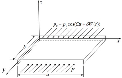
The length and width of the rectangular thin plate are and , the thickness is . The plate is simply supported and 0 and . The coordinate system is establish, as shown in Fig. 1. It is assumed that , , represent the displacement of a middle plane point of the thin plate in the , and directions. The in-plane narrow band noise excitation is imposed at 0 edge which has the expression that: , where denotes the steady pressure, means the fundamental frequency of the excitation, denotes the strength of the noise, and is unit Wiener process. The friction force [10] is imposed at edge, which is in the form of , where is the coefficient of boundary friction.
Fig. 1Model of a rectangular thin plate and the coordinate system
The transverse vibration function can be given by the von Kármán equation for the thin plate:
where is the multiple harmonic operators, is the density of thin plate, is the damping coefficient, is the bending rigidity, , is Young’s modulus, is Possion’s ratio, and is the stress function:
where , , are the components of the in-plane stress resultant. The boundary conditions are assumed to be:
The boundary condition of edge can be expressed as:
The transverse deflection of the first order modular is expressed as:
Substituting Eq. (6) into Eq. (2), and considering the boundary condition Eqs. (4), (5), the stress function can be solved, then applying Eq. (3) the internal force can be obtained:
Substituting Eq. (6) into Eq. (2), and by applying the Galerkin approach, the nonlinear vibration equation is given:
Considering the Eq. (7), the Eq. (9) can be rewritten as:
where:
Considering, , , , , , , , , then substitute the above no dimensional variables into Eq. (9) and dropping the over star yields the dimensionless function as following:
where the denotes the mark for small perturbation terms.
3. Modeling of the plate
The uniformly approximate solution of Eq. (10) is expressed in the following form:
where , are fast and slow time scale respectively.
In this study only the first-order uniform expansion of the solution is calculated. Denoting , , the ordinary-time derivatives can be transformed into partial derivatives as:
Substituting Eqs. (11), (12) into Eq. (10), and comparing coefficients of with equal powers, one obtains:
The general solution of Eq. (13) can be expressed as:
where the is the complex conjugate of its preceding terms, and is the slowly varying amplitude of the response. Substituting Eq. (12) and Eq. (14) into Eq. (13), yields:
where the over bar stands for the complex conjugate, . For Wiener process , , , one has:
We focus on the primary resonances of the system Eq. (1). Introducing the detuning parameter as follows, . One has:
Using the above Eq. (17) and eliminating the secular terms of Eq. (15) yields:
Expressing into the polar form:
Substituting Eq. (19) into Eq. (18) and separating the real and imaginary parts of Eq. (18) yields:
where , Eq. (11) is the first-order equation governing the modulation of the amplitude and phase.
The steady state response is decided by:
where and denote the steady amplitude and phase.
4. Stability
Different definitions of stochastic stability have been reported: the almost certain stability and the moment stability. Subsequently, we discuss the almost certain stability of the trivial solution by the linearizing Eq. (20) at (0, 0):
Let , Eq. (22) can be written as the following Ito equations:
The largest Lyapunov exponent of the corresponding solution is given by [11]:
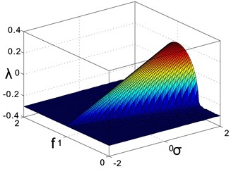
The almost certain stability of the trivial solution can be determined by the largest Lyapunov exponent , when the trivial solution is almost certainly stable. Otherwise the trivial one is almost certainly unstable. In the deterministic case when 0, as known that the Lyapunov exponent of system Eq. (10) is . Such that the trivial solution of Eq. (10) is stable if and only if . When 0.3, 0.1, the variation of with and are illustrated in Fig. 2(a), and the corresponding level lines are observed in Fig. 2(b). From Fig. 2(a) and (b), it can be seen that is a decreasing function of parameter . On the other hand is an increasing function of parameter . If the exciting frequency is located near the parametrical resonance frequency : the Lyapunov exponent rises up. In short, trivial solution stability of Eq. (10) is as same as the linear system. Hence there remains a demand that the nontrivial solutions steady state response caused by the nonlinearity should be studied.
Fig. 2a) The Lyapunov exponent, b) the corresponding level lines
a)
b)
The Floquet theory is applied to investigate the stability of the nontrivial steady state response by linearization [12].
Assuming where are the small perturbation terms, substituting the above equations into Eq. (11) and ignoring the high order terms, the linearization is expressed as:
Substituting Eq. (21) into Eq. (25) yields the Ito type stochastic equation:
where is the standard unit Gauss white noise.
It is significant to explore the stable conditions for the steady state solutions. The moment method is an effective tool [12] to estimate the steady state solutions statistically. Firstly, we take expectations on both sides of Eq. (27), considering the expectation of the Gauss white noise equals to zero, one obtains:
which yields:
The Jacoby matrix is a frequently applied approach to judge the stability of the moment, which is expressed as follows:
The characteristic equation is in the form:
where:
The roots of the Eq. (29) are:
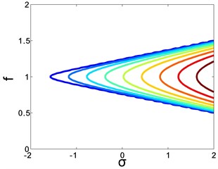
Obviously, the stable condition of the system Eq. (11) without noise is (condition 1), which demonstrates that the solution is realizable by numerical simulation. And the condition for existing complex roots is (condition 2), which means there exists periodical vibration. We can observe the bifurcation from Fig. 3.
Then we consider the second order moment of the steady state solutions since the first two order moments are of the most importance. Similarly, one has:
Applying the Ito’s rule of stochastic differentiation [13], one obtains:
Considering Eqs. (14) and (32), one obtains:
Form Eq. (33) it is easy to see that, for there must exit and . One finds that the existing condition for second order moment is the same as the stability condition for the first order moment. Then we can get the approximate probability density function of the amplitude with the form of normal distribution by Eq. (36), where denotes the mean and denotes the variance.
Fig. 3Bifurcation of the nontrivial solution with detuning frequency
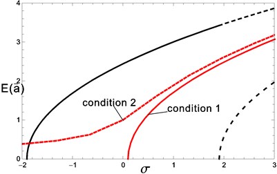
Fig. 4The amplitude frequency responses of the system (the solid line: theoretical solution, red circle: responses of noise free system, black square: responses of δ= 0.05 noise, solid black dots: responses of δ= 0.1 noise)
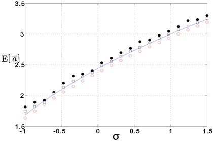
5. Numerical simulation
Letting 4, 0.3, 0.2, 0.4, 0.1, and applying the method proposed in reference [14], the numerical results of the first and second moment of Eq. (10) with are given in Fig. 4. For comparison, the deterministic solutions are also given.
As shown in Fig. 4, it is clear that the numerical results verify the theoretical analysis quite well if the density of noise is small. Now, we study the effect of the noise.
The noise free system has a stable periodical solution which is shown as a limit cycle in the Fig. 5(a), while the limit cycle is diffused by the noise as shown in Fig. 5(b)-(c). The noise changes the periodical vibration into a quasi-periodical motion. The stronger the strength of noise is, the wider the width of the limit cycle will be.
Eventually, we discuss the probability density of the steady amplitude influenced by the strength of the noise. All 1000 sets of narrow band noise with same fundamental frequency and strength are imposed to the system. The statistical results and the approximate normal distribution are both given in Fig. 6. From the simulation results, it is clear that large noise strength results in large variance.
Fig. 5The phase plot of the system
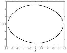
a)0
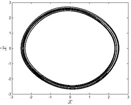
b)0.05
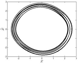
c)0.1
Fig. 6The probability density of the response (circles: numerical simulation, lines: approximate normal distribution)
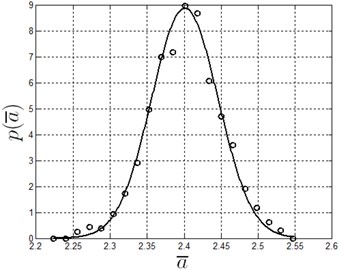
a)0.05, 0.042
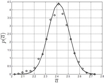
b) 0.1, 0.092
6. Conclusions
In this present paper, a rectangular thin plate excited by in-plane narrow band noise is studied. Some results are obtained as follows:
1) The stochastic stability of the trivial solution is determined by the system’s linear damping coefficient and the exciting amplitude.
2) The noise will diffuse the limit cycle of the noise free system. The width of the limit cycle is determined by the noise density. The stronger the noise strength is, the wider it will be.
3) Appling the moment method, the approximate probability density of the steady amplitude is obtained. With small enough noise density, the response is in form of the Gauss distribution. The results of the digital solution agree with the analysis.
This paper enriches the studies on the thin palate vibration problems due to the new exciting form. The nonlinear vibration research has been extended to stochastic vibrating field which has many potential applications in manufacturing, aerospace engineering and civil engineering.
References
-
Abe A., Kobayashi Y., Yamada G. Two-mode response of simply supported, rectangular laminated plates. International Journal of Nonlinear Mechanics, Vol. 33, Issue 4, 1998, p. 675-690.
-
Chang S. L., Bajaj A. K., Krousgrill C. M. Nonlinear vibrations and chaos in harmonically excited rectangular plates with one-to-one internal resonance. Nonlinear Dynamics, Vol. 4 Issue 5, 1993, p. 433-460.
-
Zhang W., Liu Z. M. Global dynamics of a parametrically and externally excited thin plate. Nonlinear Dynamics, Vol. 24 Issue 3, 2001, p. 245-268.
-
Yu P., Zhang W., Bi Q. S. Vibration analysis on a thin plate with the aid of computation of normal forms. International Journal of Nonlinear Mechanics, Vol. 36 Issue 4, 2001, p. 597-627.
-
Holmes P. J. Bifurcations to divergence and flutter in flow-induced oscillations: a finite-dimensional analysis. Journal of Sound and Vibration, Vol. 53 Issue 4, 1977, p. 161-174.
-
Holmes P. J., Marsden J. E. Bifurcations to divergence and flutter in flow-induced oscillations: an infinite-dimensional analysis. Automatica, Vol. 14 Issue 4, 1978, p. 367-384.
-
Holmes P. J. Center manifolds, normal forms and bifurcations of vector fields with application to coupling between periodic and steady motion. Physica D, Vol. 2, 1981, p. 449-481.
-
Ge G., Wang H. L., Xu J. Stochastic bifurcation for a thin rectangular plate subject to in-plane stochastic parametrical excitation. Journal of Vibration and Shock, Vol. 28, Issue 9, 2009, p. 91-94, (in Chinese).
-
Zhu Z. Z., Zhang Q. X. Xu J. Nonlinear dynamic characteristics and optimal control of giant magnetostrictive laminated plate subjected to in-plane stochastic excitation. Journal of Superconductivity and Novel Magnetism, Vol. 26, Issue 4, 2013, p. 1343-1347.
-
Ye M., Xiao X. L. Analytical Mechanics. Tianjin University Publisher, Tianjin, 2001.
-
Li J. R., Xu W., Ren Z. Z., et al. Maximal Lyapunov exponent and almost-sure stability for stochastic Mathieu-Duffing systems. Journal of Sound and Vibration, Vol. 28, Issue 6, 2005, p. 395-402.
-
Rong H. W., Xu W., Tong F. Principal response of Duffing oscillator to combined deterministic and narrowband random parametric excitation. Journal of Sound and Vibration, Vol. 210 Issue 4, 1998, p. 483-515.
-
Zhu W. Q., Lu M. Q., Wu Q. T. Stochastic jump and bifurcation of a duffing oscillator under narrow-band excitation. Journal of Sound and Vibration, Vol. 165, Issue 2, 1993, p. 285-304.
About this article

This work was supported by the National Natural Science Foundation of China (Grant No. 11402168, 11272229 and Grant No. 11302144) and Natural Science Foundation of Tianjin (Grant No. 14JCQNJC05600, 13JCYBJC17900) and the Science Foundation of Tianjin Education Committee (Grant No. 20120902).
