A contrast between classical method and finite element method for calculating strength in impeller of centrifugal pump

1. Introduction

Nowadays, the approximation methods [1-3] are generally adopted to calculate the strength of the centrifugal pump impeller. However, these methods can only roughly estimate the stress of the impeller [4], but not the stress characteristics of the precise position and the maximum stress position. Moreover, the finite element method is also adopted to perform strength calculation, but without consideration of the impact the solid movement deformation posed to the flow field, one-way coupling method leads to calculation errors. Thus, this paper use both “direct-calculation method” [5] and “the finite element method” [6] to calculate the strength of the centrifugal pump impeller. For “direct-calculation method”, it’s combined with MATLAB software to calculate the strength of the impeller’s main wheel and the side wheel. With the two-way coupling in the finite element analysis software-ANSYS, the strength of the centrifugal pump impeller rotating with the motor while buffeting by water can be fully embodied. Moreover, the impeller strength obtained by both methods meets the requirements.

2. Direct-calculation method [5]

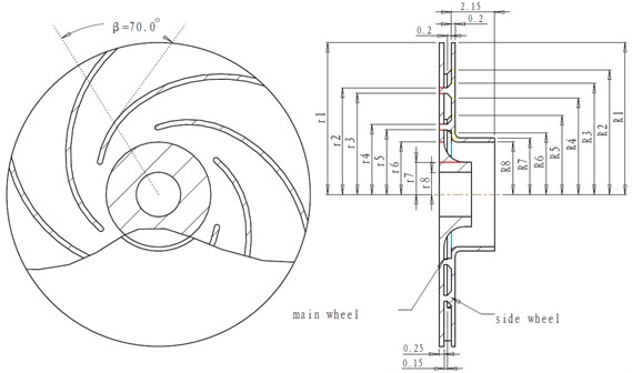
A centrifugal pump impeller whose main wheel and side wheel are both round plates with equivalent thickness is made of cast aluminum alloy; its brand is of YL108; its elongation delta is $\delta =\mathrm{}$1 %; its elastic modulus is $E=\text{70}\text{GPa}$; its Poisson’s ratio is $\mu =$0.3, ${\sigma }_s=\text{280}\text{MPa}$ and ${\sigma }_B=\text{310}\text{MPa}$, and its density is $\rho =\text{2.77}\text{g/}{\text{cm}}^{\text{3}}$ [7]. Generally, in engineering, those materials whose elongation delta $\delta$ is smaller than 5 % are referred to as brittle materials. Thus, the strength of the impeller is to be checked according to the method of brittle material [8]. The main dimensions are shown in Fig. 1, and the maximum speed is $n=$60 r/s, and the number of vane is $Z=$ 7.

1) Divide the main wheel and the side wheel into seven segments; record the original data, which is shown in Fig. 1, where $r_i(i=\text{1,}\text{…}\text{, 8})$ is used to represent each radius of 7 segments from the main wheel, which is shown in Table 1, $R_i$ ($i=$ 1,…, 8) is used to represent each radius of 7 segments from the side wheel, which is shown in Table 2, $h\left(n\right)$ is the thickness of the main wheel at radius r or the thickness of the side wheel at radius $R$, $h\left(\pi \right)=\text{3.5}\text{mm}$ is the thickness of blade, $b=\text{2.5}\text{mm}$ is the width of blade, $\beta =\mathrm{}$70° is the angle between the tangent and the diameter of the blade.

Fig. 1The impeller

2) Determine the additional load value on the vane with the Eq. (1), and 50 % of the vane weight is born by the main wheel while 30 % of the vane weight is born by the side wheel, whereas the remaining 20 % of the load is compensated by the shear stress in the blade cross section:

3) Determine the value of ${\sigma }_t$ and ${\sigma }_r$ with Eqs. (2), (3) and (4).

The boundary conditions in the outer contour of the impeller (the first loop) are as follows.

When $r=r_1$, ${\sigma }_r=$0, and ${\sigma }_t={\sigma }_0$, where ${\sigma }_0$ is the unknown hoop stress.

Determine the constant $C_1$ with the Eq. (2) and the constant $C_2$ according to the boundary conditions. Then, substitute $C_1$ and $C_2$ into the Eq. (2). It is defined that $A={\sigma }_t+{\sigma }_r\text{,}$$B={\sigma }_t-{\sigma }_r$. For the first loop, that is, at $r=r_2$, it has:

The stress of the first loop at $r_2$ is:

When $r=r_6$, the thickness between the adjacent loops mutates. In order to determine the stress of the sixth loop at $r_6$, it can be obtained by the consistency condition that:

As the impeller is loosely slipped over rather than an interference fit on the shaft, therefore, at the inner contour of $r_8$, it has ${\sigma }_r=$ 0. Based on the boundary conditions, ${\sigma }_0$ is determined by MATLAB. Then substitute ${\sigma }_0$ to the stress expression and then the stress of each loop is obtained.

Further, it’s shown graphically in Table 1 and Table 2.

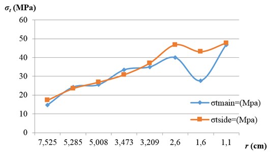
4) Draw the stress image according to the data in Fig. 1, as shown in Fig. 2.

Fig. 2The stress image of the main wheel and the side wheel of the impeller

5) Check the strength of the brittle material impeller.

The strength condition of the brittle material impeller is ${\sigma }_{\mathrm{m}\mathrm{a}\mathrm{x}}\le \left[\sigma \right]$ here $\left[\sigma \right]=\epsilon \sigma B/n_B$, and the impact factor of the absolute size (thickness) $\epsilon =$0.74, and the safety factor of strength $n_B=$4.

Thus, it can be calculated that $\left[\sigma \right]=$57.35 MPa; the maximum stress of the main wheel ${\sigma }_{\mathrm{m}\mathrm{a}\mathrm{x}\mathrm{m}\mathrm{a}\mathrm{i}\mathrm{n}}=$46.7965 MPa; the maximum stress of the side wheel ${\sigma }_{\mathrm{m}\mathrm{a}\mathrm{x}\mathrm{s}\mathrm{i}\mathrm{d}\mathrm{e}}=$47.765 MPa, all satisfying the strength condition.

3. The finite element method

In this paper, the large general finite element software-ANSYS Workbench is adopted to analyze the fluid structure coupling of impeller and water [9, 10]. First, analyze the flow field with ANSYS CFX and get the water pressure on the impeller. Then, substitute the data to the statics analysis module and determine the stress and deformation of the impeller. Finally, substitute the data to modal analysis and obtain the first eight modes of the impeller [11].

3.1. The establishment of a 3D model and the extraction of the flow channel

As shown in Fig. 3, the 3D model of impeller is established by the 3D drawing software-CREO 2.0. Then, it is imported into ANSYS workbench to create a Geometry, and after that the flow channel is extracted utilizing the command “fill” in the Design Modeler, as shown in Fig. 4.

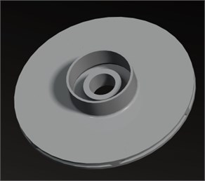
Fig. 3The impeller

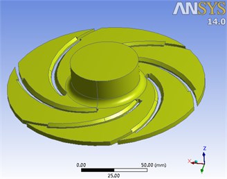
Fig. 4The flow channel

3.2. Fluid-structure coupling of the impeller

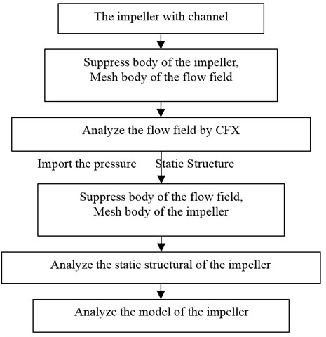
Fluid-structure interaction analysis of the impeller was conducted through ANSYS Workbench, and the process is shown in Fig. 5 [12].

Fig. 5Flow chart

3.2.1. The flow field analysis

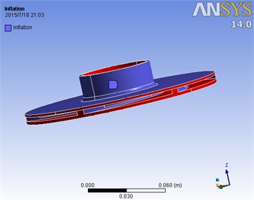
When analyzing the flow field, suppress body of the impeller first. Then, the body of the flow field is meshed with the element size of 2 mm, and the main surface of the flow field is set as boundary of 3 layers. Based on the tetrahedral meshing method, the flow field is meshed to 173579 elements in total, the mesh diagram of the flow field is shown in Fig. 6 and the inflation of it is shown in Fig. 7.

Fig. 6The meshing diagram of the flow

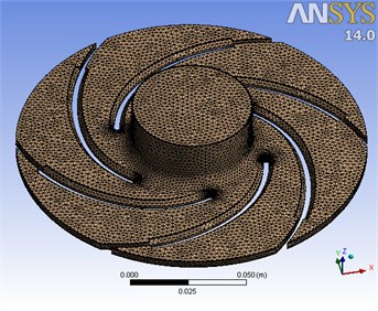
Fig. 7The inflation of the impeller

Then, define the boundary condition of the inflow-port and the outflow-port as “inlet” and “outlet”, respectively, whereas the normal speed is 2.65 m/s and the relative pressure is 1 atmosphere. Moreover, define the boundary condition of all the surfaces except inflow-port and outflow-port as “wall”, as shown in Fig. 8. After that, start running until the solutions are convergent. From the velocity streamline of the flow field (Fig. 9), it can be seen that the flow velocity on the pressure surface increases gradually with the increasing of the radius, and reaches the maximum near the inflow-port. Meanwhile, from the pressure figure of the flow field (Fig. 10), it can be seen that the maximum pressure is in the inflow-port of the impeller, and decreases with the water being thrown away by the centrifugal force.

Fig. 8Define the boundary condition of the flow field

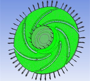
Fig. 9The velocity streamline of the flow field

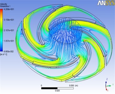
Fig. 10The pressure figure of the flow field

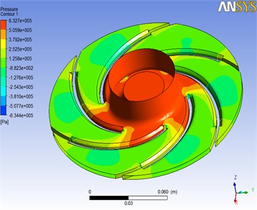
Fig. 11The meshing diagram of the impeller

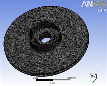
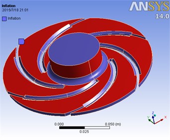
Fig. 12The inflation of the impeller

3.2.2. Impeller structure statics analysis

In engineering materials database of ANSYS Workbench, aluminum alloy is selected to suppress body of the flow field except the solid impeller. Then, the body of the impeller is meshed with the element size of 1.5 mm, and the main surface of the impeller is set as boundary of 3 layers. Based on the automatic meshing method, the impeller is meshed to 255439 elements in total. The mesh diagram of the impeller is shown in Fig. 11 and the inflation of it is shown in Fig. 12.

Fig. 13The imported impeller pressure

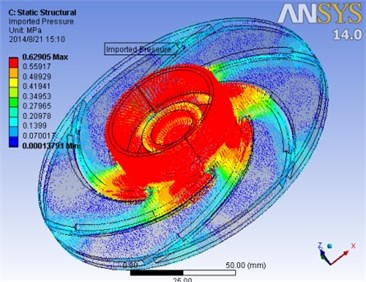
The solution of the fluid flow (CFX) is imported to the Static Structure, with the imported impeller pressure as shown in Fig. 13. Then, define the rotation velocity on the center axis of the impeller as 60 r/s, and add a fixed support on the inflow-surface to solve the structural statics.

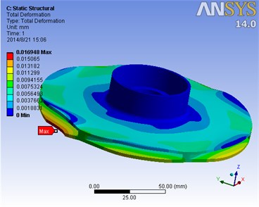
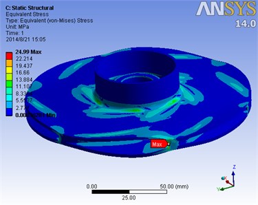
The results of the finite element analysis are shown in Fig. 14, and the maximum stress and the total deformation of the impeller can be known from it. It can be seen that the maximum total deformation of 1.6948 e-002 mm appears in the outside diameter of the main impeller, as marked in the figure. According to the fourth strength theory, the maximum equivalent stress is 24.99 MPa, which appears in the tail-end blade, as marked in the figure [13].

Fig. 14Results of the finite element analysis

3.2.3. Impeller modal analysis

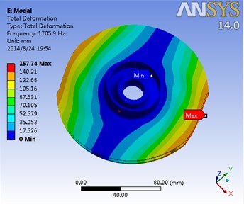
Modal analysis is a very effective method to avoid the potential resonance of the impeller. Without considering gravity, the modal analysis of hydraulic loading and rotation is conducted with the final data of fluid-solid coupling being introduced. Moreover, the first eight order modes of impeller and its corresponding frequency are shown in Fig. 15. Meanwhile, it is shown in Table 3 the results of the impeller modal analysis of the flow field.

Table 3The results of the impeller modal analysis in the flow field (Hz)

Mode	1	2	3	4	5	6	7	8
Frequency	1705.9	1706	2043.5	2245.4	2245.5	3233.9	4010.7	5071.1

Fig. 15The first eight order modal of the impeller and the corresponding frequency

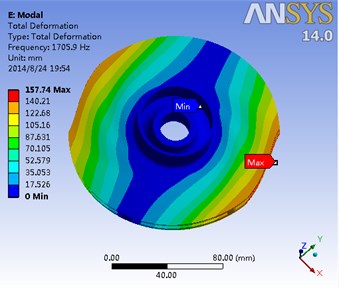
a) First-order mode frequency1705.9 Hz

b) Second-order mode frequency 1706 Hz

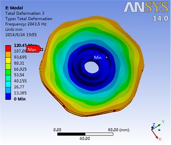
c) Third-order mode frequency 2043.5 Hz

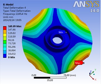
d) Fourth-order mode frequency 2245.4 Hz

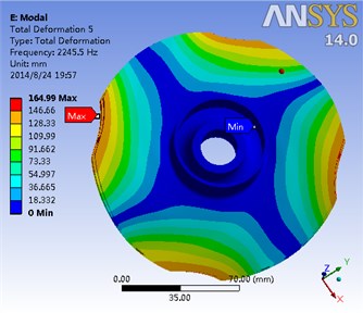
e) Fifth-order mode frequency 2245.5 Hz

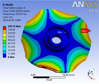
f) Sixth-order mode frequency 3233.9 Hz

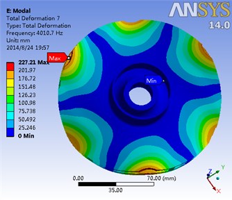
g) Seventh-order mode frequency 4010.7 Hz

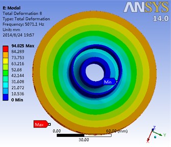
h) Eighth-order mode frequency 5071.1 Hz

4. Conclusion

The maximum stress calculated by the fluid-structure coupling to impeller and the flow field is less than that obtained by the “once calculation method”. The method of fluid-structure coupling concerns about the pressure of the fluid flow on the impeller while combining with the structure statics by using the two-way coupling to get the final stress. However, for the traditional “once calculation method”, only the structure statics is used and only the average stress is considered which can hardly know the stress concentration source. Even if it is considered that the plastic deformation of the stress concentration areas is intensified, the strength checking of these areas still cannot be slackened. Thus, based on the comparison between the results of the two methods, it’s more comprehensive and reliable to utilize the finite element method. Therefore, it is demonstrated that in the practical production design and checking, more rigorous and efficient data and higher safe reliability of the impeller operation can be realized by combining the conventional computation method with the finite element method.