Abstract
This study develops an automatic prediction model for ground vibration induced by Taiwan high-speed trains on embankments. Various field-measured ground vibration data comprise a database used for developing the prediction model. First, the main characteristics that affect the overall vibration level are established on the basis of measurement result database. These main influence factors include train speed, ground condition, measurement distance, and supported structure. A support vector machine (SVM) algorithm, which is a widely used classification model, is then adopted to predict the vibration level induced by high-speed trains on embankments. The measured and predicted vibration levels are compared to verify prediction model reliability. Analytical results show that the more the measured vibration data located in one vibration group is collected, the higher of the accuracy rate will be. Generally, the developed SVM model can reasonably predict ground vibration level in various frequency ranges. Prediction results are discussed in detail, and the methodology for developing the automatic ground vibration level prediction system is presented.
1. Introduction
High-speed rail is a type of rail transport that operates significantly faster than traditional rail traffic owing to the use of an integrated system of specialized rolling stock and dedicated tracks. Given that high-speed rail guarantees environmental, economic, and transportation benefits, many countries have developed such systems to connect major cities. However, experience shows that the ground vibration induced by trains can potentially disrupt vibration-sensitive operations in such facilities as hospitals, laboratories, and low-vibration fabrication facilities. These facilities often contain equipment that can be affected by minimal ground vibration levels. Hence, ground vibrations induced by high-speed trains have drawn considerable research interest in recent years. Measurement techniques have thus been studied, and vibration characteristics have been evaluated to develop a vibration mitigation scheme.
To evaluate the possible vibration level, a prediction methodology for ground vibration induced by high-speed trains on various structures has been developed [1-3]. Based on these suggestions, the main factors that affect vibration levels can be grouped into vibration source, vibration path, and vibration receiver. Many authors [4-6] used numerical analysis to study rail systems with various structure types. Research on this subject has progressed well in the past several decades. Moreover, some researchers [7-10] have studied ground vibration characteristics using field measurement data.
On the basis of the ground vibration measurements of possible influence factors for near- and far-field vibrations, numerous authors [2, 3, 10] have concluded that structure type, train speed, ground condition, and frequency dependence are the most important factors in evaluating the ground vibration behavior of high-speed trains. Chen et al. [7, 8] recently measured the ground vibration induced by Taiwan high-speed trains on embankments to evaluate the characteristics of near-field vibration and the propagation of far-field vibration.
Developing a relatively simple and automatic prediction model to help engineers improve the accuracy of preliminary analysis is essential since existing methods in design manuals are not sufficient to reflect the complicated behavior. The main objective of this study is to propose an automatic ground vibration prediction model for high-speed trains. This prediction model is based on a systematic understanding of ground vibration characteristics which are performed in previous studies.
Extensive ground vibration measurement data from Taiwan high-speed trains on embankments are used in this study to establish the vibration characteristics. A widely used prediction model called the support vector machine (SVM) technique is applied on the basis of these influence characteristics. The measured and predicted vibration levels are compared to verify prediction model reliability. The analysis results are discussed in detail, and the methodology for developing an automatic prediction system for ground vibration level induced by high-speed trains is presented.
2. Analysis method
Various techniques can be used to characterize vibration measurement data levels and to predict possible ground vibration level. To address these techniques, the ground vibration analysis method and SVM classification model are briefly discussed below.
2.1. Ground vibration
For most sensitive equipment, manufacturers provide detailed criteria that define acceptable vibration level. These criteria are usually frequency-dependent, thus reflecting the vibration sensitivity of the internal components of an instrument. Based on the ground vibration characteristics induced by high-speed trains, a range of amplitudes (10 dB to 100 dB, ref. 1 micro-inch/sec) and frequencies (1 Hz to 100 Hz) are required to assess ground vibration. A frequency domain of 1/3 octave band for the center frequency range of 1 Hz to 100 Hz is adopted to describe the vibration level in dB and to evaluate the frequency effect. Ground vibration level is expressed in terms of the root-mean-square (RMS) velocity of the ground vibration level, which is defined in dB as follows:
where is the vibration level, is the measured velocity, and is the referred velocity (2.54×10⁻⁸ m/sec).
The overall vibration level is often used to evaluate the total vibration energy (e.g., [2, 7, 11]), and this parameter can be transferred from the RMS velocity of each 1/3 octave band vibration level, as shown in the calculation below:
where is the overall vibration level in dB, is the central frequency of each 1/3 octave band, and is the vibration level of each frequency of the 1/3 octave band.
2.2. Prediction model
For ground vibration prediction, the SVM algorithm is adopted to classify high-speed trains-induced vibration levels because this approach is probably the most widely used kernel learning algorithm [12]. The analysis of the SVM algorithm is mainly based on the vibration measurement database characteristics.
The basic concept of SVM is the application of nonlinear mapping from an input space to a high-dimensional feature space using a linear model to form a decision boundary. For a given training set {(, ), (, ),…, (, )}, , , where is a -dimensional sample vector, and denotes the class labels of , the supposed optimal separating hyperplane not only separates the two classes but also maximizes the margin between the classes if the samples are linearly separable. The hyperplane is written as:
where denotes the inner product, denotes the normal vector to the hyperplane, and is the distance from the origin to the hyperplane along the normal vector. The margin can be defined as:
The task of maximizing the margin can be summarized as:
Lagrange theory is used to solve the problem, which is defined as:
where (,,..., ) is the vector of the Lagrange multipliers, and , 0, 1, 2,..., .
When the classes are not linearly separable, a new set of variables is introduced, namely:
where the variables 0, 1, 2,…, , are the slack variables. is the total amount by which constraints are violated. The slack variables are added to handle non-separable cases. Thus, should be as small as possible for optimization.
This classifier is nonlinear in the original features but is linear in the expanded feature space. is replaced by for some nonlinear , such that the decision boundary is a nonlinear surface. SVMs do not produce a dot product in a high-dimensional feature space. These products are replaced with a kernel function instead. The kernel function is a symmetric positive definite function that satisfies Mercer’s condition of 0. Function is analogous to a nonnegative definiteness for a matrix. Solve the optimization problem is easier using:
The most commonly used kernel function is the Gaussian radial basis function (RBF):
where is the kernel parameter.
3. Database for analysis
3.1. Background of high-speed trains
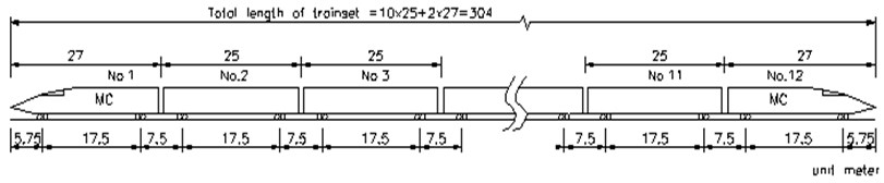
The trainset configuration and the related dimensions of Taiwan high-speed trains are shown in Fig. 1. Each Taiwan high-speed trainset consists of 12 train cars, where 10 cars are passenger cars and two locomotive cars. Each passenger car (PC) is 25 m long, whereas each locomotive car is 27 m long. Thus, the total length of the trainset is 304 m, as shown in Fig. 1.
Fig. 1Configuration of trainset for the Taiwan high-speed rail
3.2. Ground vibration measurement
The main measuring equipment consisted of accelerometers, integrator, and a data acquisition system. The following procedure is used for installing sensors to attach the ground:
a) Excavate a pit with proper dimensions which can install accelerometers.
b) Place the standard sand on the bottom of pit to even the excavated surface.
c) Compact the excavated surface and assure the surface in the horizontal level.
d) Place firmly accelerometers, which connect a steel plate as a firm base, on the ground.
e) Set the accelerometer direction: the -direction is in the train passing; the -direction is perpendicular to the train passing; and the -direction is for the direction of gravity.
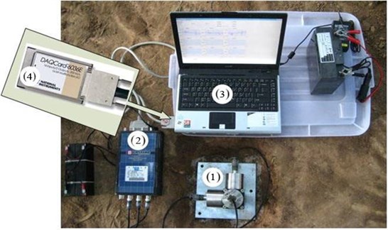
A set of measuring instruments and equipment for this study is shown in Fig. 2. The measured vibration accelerations included -- directions. Only the vertical component ( direction) is used in the subsequent discussion to simplify the process of vibration impact assessment.
Fig. 2Measuring equipment: (1) accelerometers, (2) integrator, (3) and (4) data acquisition system
The vibration measuring plan includes near-field and far-field measurements. The distance of the near-field vibration was set beside the alignment of high-speed trains. For far-field measurement, additional three measurement points in each site, which were in a straight line and perpendicular to the alignment of high-speed trains, are used to simultaneously measure the ground vibration when trains pass through the specific location. Fig. 3 shows the schematic diagram of embankment and a typical schematic layout of the measurement points. All these measurement points were employed to simultaneously measure the ground vibration when trains pass through the specific location. Before measuring, all equipment must be synchronized.
Fig. 3Schematic diagram of embankment and typical schematic layout of measurement site
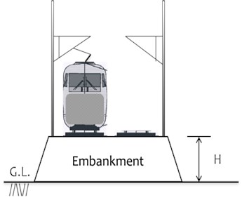
a) Schematic diagram of embankment
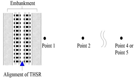
b) Schematic measurement layout
The series of measurements performed in this study comprises different factors, such as geological conditions, embankment heights, and train speeds. Table 1 lists the basic information of these measurement sites. The measurement distances ( to ) are 22 m to 203 m from the track center, and the selected embankments have various heights that range from 3.6 m to 6.8 m.
The geological conditions include sand/silt/clay soils, gravel, and rock. These conditions range from soft ground to hard ground. Ground shear wave velocity () is used as an indicator to describe soil stiffness. The value increases with increasing soil stiffness. The average taken from the ground surface to 10 m in depth ranges from 170 m/s to 650 m/s, which is representative of the surface wave analysis. Table 1 evidently shows that various geological conditions and ground shear wave velocities are covered.
Table 1Basic information of measurement sites
Site No. | Soil type | (m) | (m/s) | (m) | (m) | (m) | (m) |
1 | Silty clay | 5.3 | 170 | 28 | 53 | 78 | 101 |
2 | Sandy silt | 5.2 | 230 | 33 | 68 | 93 | 118 |
3 | Gravel | 3.6 | 430 | 36 | 69 | 149 | 203 |
4 | Sandstone | 6.8 | 650 | 22 | 47 | 122 | 202 |
– height of embankment from ground level (G.L.); – ground shear wave velocity; – measurement distance from track center | |||||||
3.3. Ground vibration characteristics
The measured results of ground vibration are shown in Table 2. Based on field measurements, the main characteristics that influence vibration levels include geological conditions, attenuation distance, and train speed. Fig. 4 presents the relationships of the overall vibration level with the train speed, ground shear wave velocity, and measurement distance. Evidently, the vibration level increases with the train speed. However, the vibration level decreases as the ground shear wave velocity and measurement distance increase.
Table 2Measurement results of ground vibration
Site | (m/s) | Speed (km/h) | ||||||||||||||||
VL-Z-axis (dB) | VL-Z-axis (dB) | VL-Z-axis (dB) | VL-Z-axis (dB) | |||||||||||||||
VLOA | VLL | VLM | VLH | VLOA | VLL | VLM | VLH | VLOA | VLL | VLM | VLH | VLOA | VLL | VLM | VLH | |||
1 | 170 | 150 | 65.7 | 47.9 | 51.7 | 64.5 | 49.5 | 45.4 | 44.3 | 44.4 | 50.6 | 49.7 | 40.4 | 40.2 | 52.8 | 52.0 | 43.4 | 40.6 |
170 | 170 | 66.6 | 45.9 | 48.1 | 65.6 | 56.6 | 55.9 | 43.3 | 46.2 | 55.7 | 55.4 | 40.8 | 41.0 | 52.0 | 51.5 | 39.1 | 39.3 | |
170 | 180 | 64.8 | 45.9 | 48.1 | 65.6 | 49.6 | 45.8 | 44.6 | 43.8 | 50.5 | 49.5 | 41.1 | 39.8 | 52.1 | 51.3 | 42.8 | 39.3 | |
170 | 190 | 65.0 | 44.5 | 48.6 | 66.5 | 50.5 | 47.7 | 44.4 | 44.0 | 50.0 | 49.2 | 40.1 | 38.6 | 48.7 | 47.1 | 41.8 | 38.4 | |
170 | 200 | 65.7 | 49.7 | 50.8 | 64.8 | 53.0 | 47.3 | 47.1 | 49.8 | 51.3 | 47.4 | 45.8 | 46.4 | 51.7 | 47.3 | 47.9 | 44.9 | |
170 | 210 | 64.8 | 47.4 | 51.8 | 64.4 | 49.9 | 46.8 | 43.3 | 44.7 | 48.8 | 47.7 | 39.9 | 38.6 | 47.9 | 46.1 | 41.6 | 38.2 | |
170 | 290 | 65.1 | 55.7 | 46.3 | 67.7 | 54.5 | 51.7 | 45.7 | 49.8 | 56.1 | 52.9 | 51.9 | 47.3 | 55.2 | 53.0 | 48.3 | 47.9 | |
170 | 300 | 64.8 | 49.7 | 50.8 | 64.8 | 54.0 | 51.4 | 45.6 | 49.0 | 56.1 | 52.6 | 52.0 | 48.3 | 55.1 | 52.8 | 49.2 | 47.1 | |
170 | 300 | 65.1 | 47.4 | 51.8 | 64.4 | 52.8 | 46.8 | 46.7 | 49.9 | 50.8 | 47.2 | 45.5 | 45.3 | 51.3 | 46.9 | 47.4 | 44.9 | |
2 | 230 | 200 | 68.7 | 53.5 | 57.2 | 68.2 | 54.9 | 51.3 | 51.9 | 43.5 | 54.0 | 51.6 | 49.1 | 43.9 | 52.9 | 52.5 | 42.4 | 35.1 |
230 | 280 | 68.4 | 51.1 | 62.4 | 67.0 | 62.1 | 50.6 | 61.6 | 46.7 | 59.7 | 54.9 | 57.7 | 46.2 | 57.5 | 51.8 | 56.0 | 40.0 | |
230 | 290 | 69.8 | 54.7 | 59.1 | 69.2 | 58.8 | 51.3 | 57.1 | 50.9 | 57.1 | 53.7 | 52.3 | 50.2 | 56.5 | 55.3 | 49.6 | 41.8 | |
230 | 290 | 69.3 | 50.4 | 62.8 | 68.1 | 62.8 | 52.0 | 62.3 | 47.0 | 60.2 | 55.7 | 57.8 | 47.7 | 57.3 | 52.3 | 55.5 | 41.6 | |
230 | 290 | 69.9 | 50.7 | 62.0 | 69.0 | 63.0 | 50.8 | 62.6 | 47.6 | 59.6 | 54.1 | 57.7 | 48.1 | 56.9 | 52.8 | 54.5 | 41.9 | |
230 | 300 | 70.3 | 54.5 | 59.2 | 69.8 | 58.0 | 51.3 | 56.1 | 49.3 | 58.7 | 54.5 | 55.3 | 50.7 | 55.1 | 53.3 | 49.9 | 41.0 | |
230 | 300 | 70.7 | 54.4 | 57.9 | 70.4 | 58.7 | 52.1 | 56.8 | 50.2 | 58.1 | 55.0 | 53.7 | 49.8 | 55.7 | 54.7 | 48.2 | 40.5 | |
230 | 300 | 70.1 | 54.1 | 58.4 | 69.7 | 58.1 | 51.8 | 56.0 | 50.0 | 58.8 | 54.5 | 55.8 | 50.0 | 54.5 | 52.9 | 48.8 | 41.0 | |
3 | 430 | 280 | 66.8 | 49.8 | 64.3 | 65.1 | 55.8 | 49.1 | 52.1 | 51.4 | 50.2 | 47.7 | 46.6 | 32.1 | 49.3 | 47.2 | 44.4 | 36.9 |
430 | 280 | 69.9 | 52.7 | 70.2 | 66.0 | 57.0 | 51.6 | 52.8 | 52.3 | 54.2 | 50.6 | 50.5 | 45.7 | 53.2 | 51.0 | 48.6 | 38.4 | |
430 | 285 | 69.9 | 48.2 | 66.3 | 69.8 | 56.1 | 47.6 | 50.7 | 53.6 | 49.8 | 46.0 | 47.1 | 36.4 | 50.2 | 46.3 | 47.4 | 38.5 | |
430 | 290 | 67.5 | 50.8 | 66.6 | 63.8 | 56.5 | 49.8 | 53.6 | 50.8 | 50.5 | 48.4 | 46.2 | 32.5 | 51.3 | 48.8 | 47.1 | 38.7 | |
430 | 290 | 65.9 | 47.5 | 64.7 | 62.7 | 55.9 | 47.4 | 53.0 | 51.2 | 48.3 | 44.7 | 45.5 | 32.8 | 49.1 | 45.4 | 45.9 | 38.9 | |
430 | 290 | 69.4 | 48.5 | 66.2 | 68.3 | 56.1 | 47.8 | 50.9 | 53.5 | 49.8 | 45.2 | 47.7 | 36.6 | 50.6 | 46.2 | 48.1 | 39.0 | |
430 | 300 | 69.8 | 52.7 | 65.5 | 69.1 | 57.2 | 52.4 | 50.6 | 53.7 | 53.5 | 51.9 | 48.1 | 36.4 | 52.4 | 50.3 | 47.7 | 38.6 | |
430 | 300 | 67.4 | 51.2 | 66.8 | 63.0 | 57.5 | 50.6 | 55.0 | 51.2 | 50.3 | 47.5 | 46.9 | 33.1 | 50.6 | 48.5 | 45.6 | 38.3 | |
4 | 650 | 195 | 57.8 | 46.6 | 55.8 | 52.7 | 54.4 | 50.7 | 51.3 | 43.8 | 48.6 | 45.6 | 44.9 | 36.5 | 46.7 | 43.1 | 43.0 | 38.0 |
650 | 240 | 58.3 | 51.5 | 56.2 | 50.8 | 55.6 | 50.9 | 53.6 | 41.2 | 50.3 | 46.8 | 47.5 | 35.7 | 45.0 | 41.9 | 40.2 | 37.5 | |
650 | 245 | 58.2 | 54.0 | 54.8 | 50.5 | 56.0 | 52.7 | 53.1 | 40.6 | 49.5 | 45.2 | 47.1 | 36.2 | 46.9 | 43.6 | 43.2 | 37.0 | |
650 | 250 | 56.5 | 49.8 | 54.3 | 49.3 | 56.7 | 53.4 | 53.6 | 43.3 | 50.0 | 46.6 | 46.8 | 37.4 | 47.6 | 45.3 | 42.4 | 37.7 | |
650 | 255 | 57.0 | 48.1 | 54.6 | 51.7 | 53.3 | 48.8 | 50.8 | 42.0 | 51.0 | 48.2 | 47.5 | 35.3 | 45.3 | 42.9 | 39.7 | 36.9 | |
650 | 280 | 59.7 | 47.3 | 56.4 | 56.5 | 57.1 | 49.8 | 55.7 | 47.4 | 51.9 | 49.2 | 48.0 | 38.2 | 46.9 | 44.0 | 42.0 | 39.3 | |
650 | 285 | 60.5 | 47.5 | 57.0 | 57.5 | 57.0 | 50.0 | 55.5 | 46.6 | 52.3 | 49.5 | 48.7 | 39.0 | 47.3 | 44.7 | 41.5 | 39.8 | |
650 | 300 | 60.2 | 47.9 | 58.8 | 53.4 | 54.4 | 47.7 | 52.8 | 44.6 | 53.5 | 45.6 | 52.6 | 37.7 | 49.0 | 42.4 | 47.2 | 40.1 | |
650 | 300 | 59.8 | 45.8 | 58.7 | 52.4 | 51.9 | 46.2 | 49.0 | 45.2 | 51.3 | 44.7 | 49.9 | 38.5 | 48.4 | 40.6 | 46.1 | 42.5 | |
650 | 300 | 59.1 | 48.1 | 57.5 | 52.6 | 52.5 | 45.9 | 50.5 | 44.1 | 51.1 | 44.2 | 49.9 | 37.8 | 47.8 | 40.1 | 46.1 | 39.5 | |
Note: VLL = VLLOW; VLM = VLMIDDLE; VLH = VLHIGH | ||||||||||||||||||
Fig. 4Relationships of VLoa and various influence factors
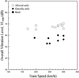
a) Train speed
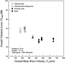
b) Shear wave velocity
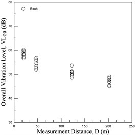
c) Measurement distance
4. Automatic prediction system
4.1. Prediction methodology
As mentioned in Section 2.2, the SVM kernel method is a supervised learning model that is popular for training known features. To construct such classification model, positive and negative data classes are provided in advance as training examples, after which a trained SVM model is constructed according to the selected features.
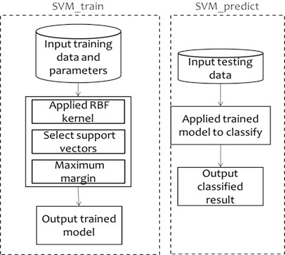
An SVM clustering tool (LIBSVM) is adopted in this study. The SVM_train and SVM_predict module in LIBSVM toolset developed by Lin’s lab [12, 13] are applied to train and classify train-induced vibration levels. An overview of SVM_train and SVM_predict module are presented in Fig. 5. In SVM_train module, all training data with defined features are trained to construct the trained model. In SVM_predict module, testing data were classified also by the previous model. The following sections discuss in detail the selection of classification features, the evaluation of different kernel transformation techniques, and the prediction results according to benchmark datasets.
Fig. 5LIBSVM’s training and predicting tool
4.2. Prediction process
Ground shear wave velocity, train speed, and measurement distance are the features for the SVM model used in this research. In this study, the RBF kernel type performs the best accuracy compared to other kernel types. Thus, the RBF is selected as the kernel type, and the function of multiclass classification is employed in this system. Based on the measured results of the possible minimum and maximum vibration levels, the SVM model output is classified into five groups of vibration level, as shown in Table 3. The vibration levels for Groups 1 to 5 are 30 dB to 40 dB, 40 dB to 50 dB, 50 dB to 60 dB, 60 dB to 70 dB, and more than 70 dB, respectively.
Table 3Group of ground vibration level
Group no. | 1 | 2 | 3 | 4 | 5 |
Vibration level (dB) | 30-40 | 40-50 | 50-60 | 60-70 | More than 70 |
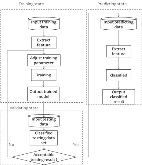
The training and prediction processes are presented in Fig. 6. In the training state, the system begins by reading the input data and then progresses to extracting and normalizing the same data to region (0, 1). The data transformed to a normal form are then entered by the system to LIBSVM, after which the training process begins. Train speed, ground shear wave velocity, and measurement distance is adopted as training and prediction features. The system uses a 10-fold cross validation. One fold is chosen as the validating fold, whereas the others are the training folds to build the hyperplane used in the validations. If testing results are better than the earlier outputs, the parameter is changed. This process is repeated several times until the system finds the result in the local maximum. The LIBSVM’s grid.py toolset is applied to implement the optimal parameters selection process. After completing the training process, the system uses a hyperplane to predict and classify the vibration level.
Fig. 6SVM prediction process
5. Prediction results
The evaluation criteria, including the accuracy rate and precision rate of the classified result, are used to evaluate the classification quality of the proposed SVM model. The accuracy rate is the percentage of the test set samples that are correctly classified by the model. Meanwhile, the precision rate refers to the percentage that classifiers labeled as positive are actually positive. The definitions are shown as follows:
where 1, 2,…, , is total number of groups.
Table 4Accuracy rate for various predicted frequency ranges
Type of frequency range | Low | Middle | High | Overall |
Accuracy rate | 0.80 | 0.82 | 0.85 | 0.76 |
Table 4 presents the prediction results of ground vibration level using the aforementioned prediction process. Analysis results show that the accuracy rates are 80 %, 82 %, 85 %, and 76 % for the low, middle, high, and overall frequency ranges, respectively. The SVM optimal training parameters include the cost parameter of 1 and gamma parameter of 0.000699, 0.000428, 0.000699, and 0.000428 for the low, middle, high, and overall frequency ranges, respectively. Thus, the developed SVM model can reasonably predict ground vibration with an accuracy rate of 76 % to 85 % in general. To improve the accuracy rate, more measured data are required in the subsequent measurement.
6. Discussion of prediction results
In the field of machine learning, a confusion matrix, which is also known as a contingency table or an error matrix [14], is a specific table layout that enables the visualization of the performance. All correct predictions are located in the diagonal of the table, thus, visually inspecting the table for errors is easy because these errors are represented by the values outside the diagonal. Table 5 shows the confusion matrix of the actual and classfied vibration levels for the low frequency range. Although only two groups of vibration levels exist at a low frequency, the results are acceptable because the values in the diagonal are relatively greater than those outside the diagonal. Table 6 shows the confusion matrix of the actual and classfied vibration levels for the middle frequency range. Grouping only occurs to misclassify to the nearby groups. Most of the vibration levels are located in Groups 2 and 3.
Table 7 shows the confusion matrix of the actual and classfied vibration results for the high frequency range. The confusion matrix reveals that even when the system misclassifies the vibration level to the wrong group, this level is still within a nearby group. Table 8 shows the confusion matrix of the actual and classfied vibration results for the overall frequency range. The results show that the system performs best in Group 3, which is also the biggest group in the vibration level of the overall frequency range.
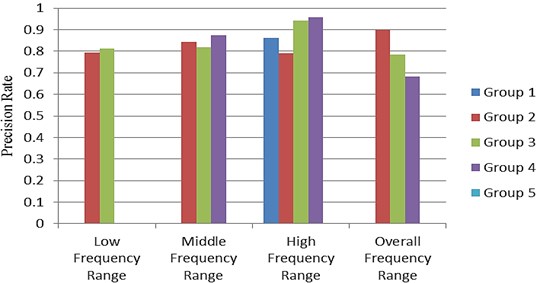
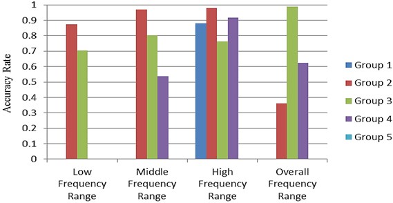
According to Tables 5 to 8, most of the vibration levels are located in Groups 2 and 3, thus, the system can separate these two groups and the other vibration level groups quite well. The vibration data in Groups 1, 4, and 5 are more likely to be misclassified because of insufficient sampling. Fig. 7 shows the number of vibration level groups in the low, middle, high, and overall frequency ranges. Fig. 8 shows the number of vibration level groups that are classified by the system in the low, middle, high, and overall frequency ranges. Fig. 9 shows the precision rate of the predicted results in the low, middle, high, and overall frequency ranges. The result shows that the precision rate of the predicted result is in the 0.78 to 0.94 region. Fig. 10 shows the accuracy rate of the predicted results in the low, middle, high, and overall frequency ranges. Based on Figs. 7 and 10, the results demonstrate that more vibration level data in a group indicates a higher accuracy rate for that group.
Table 5Confusion matrix of actual and classfied vibration results for low frequency range
Group 2 (classfied) | Group 3 (classfied) | |
Group 2 (actual) | 69 | 10 |
Group 3 (actual) | 18 | 43 |
Table 6Confusion matrix of actual and classfied vibration results for middle frequency range
Group 1 (classfied) | Group 2 (classfied) | Group 3 (classfied) | Group 4 (classfied) | Group 5 (classfied) | |
Group 1 (actual) | 0 | 3 | 0 | 0 | 0 |
Group 2 (actual) | 0 | 63 | 4 | 0 | 0 |
Group 3 (actual) | 0 | 11 | 45 | 0 | 0 |
Group 4 (actual) | 0 | 0 | 6 | 7 | 0 |
Group 5 (actual) | 0 | 0 | 0 | 1 | 0 |
Table 7Confusion matrix of actual and classfied vibration results for high frequency range
Group 1 (classfied) | Group 2 (classfied) | Group 3 (classfied) | Group 4 (classfied) | Group 5 (classfied) | |
Group 1 (actual) | 37 | 5 | 0 | 0 | 0 |
Group 2 (actual) | 6 | 45 | 1 | 0 | 0 |
Group 3 (actual) | 0 | 5 | 16 | 0 | 0 |
Group 4 (actual) | 0 | 2 | 0 | 22 | 0 |
Group 5 (actual) | 0 | 0 | 0 | 1 | 0 |
Table 8Confusion matrix of actual and classfied vibration results for overall frequency range
Group 2 (classfied) | Group 3 (classfied) | Group 4 (classfied) | Group 5 (classfied) | |
Group 2 (actual) | 9 | 16 | 0 | 0 |
Group 3 (actual) | 1 | 83 | 0 | 0 |
Group 4 (actual) | 0 | 7 | 15 | 2 |
Group 5 (actual) | 0 | 0 | 7 | 0 |
Fig. 7Number of vibration level located in various frequency ranges
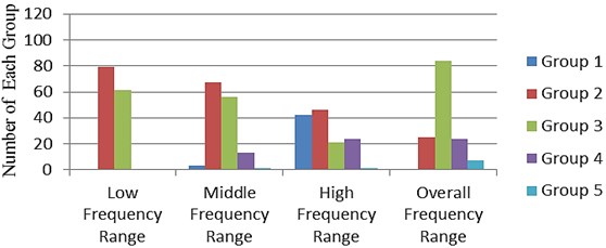
Fig. 8Number of vibration level been classified in various frequency ranges
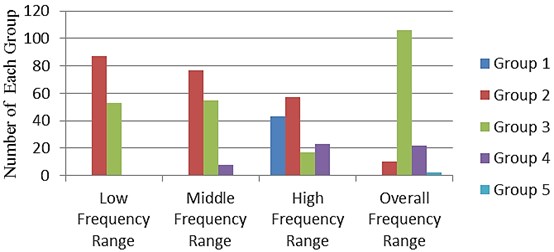
Fig. 9Precision rate of predicted results in various frequency ranges
7. Conclusions
A comprehensive field measurement data of high-speed trains on embankments are used to establish ground vibration characteristics. The main characteristics that affect the overall ground vibration are train speed, ground condition, measurement distance, and supported structure.
An automatic ground vibration prediction model using the SVM technique is developed according to these characteristics. The methodology for developing an automatic prediction system for vibration levels induced by high-speed trains has been proposed in this study. The developed SVM model can reasonably classify the vibration group with an accuracy rate of 76 % to 85 % for four types of vibration groups, including the overall, low, middle, and high frequency ranges. The validation results show that when the system misclassifies a vibration level to the wrong group, this vibration level is still in the nearby group that is, in one level of a higer or a lower group. The test results also indicated that if more measurement data in certain vibration level group, a higher accuracy rate will be obtained in that group.
Fig. 10Accuracy rate of predicted results in various frequency ranges
The automatic ground vibration prediction model for high-speed trains are important for engineers to predict possible vibration effects during the planning or preliminary design stage since existing methods in design manuals are not sufficient to reflect the complicated behavior. The proposed model in this study can help engineers improve ground vibration impact prediction and is suitable for application to a large number of assessments. The proposed prediction model is suitable to predict ground vibration induced by high speed rail riding on embankments with train speed from 150 km/h to 300 km/h, ground shear wave velocity form 170 m/s to 650 m/s and the distance to high speed rail from 22 m to 203 m from the track center. A larger amount of field measurement data are required to improve the accuracy of this automatic prediction system.
References
-
High-Speed Ground Transportation Noise and Vibration Impact Assessment. U.S. Department of Transportation, Federal Railroad Administration, Report Number 293630-1, 1998.
-
Transit Noise and Vibration Impact Assessment. U.S. Department of Transportation, Federal Transit Administration, Office of Planning and Environment, Report Number FTA-VA-90-1003-06, 2006.
-
Chen Y. J., Ju S. H., Ni S. H, Shen Y. J. Prediction methodology for ground vibration induced by passing trains on bridge structures. Journal of Sound and Vibration, Vol. 302, Issue 4-5, 2007, p. 806-820.
-
Ju S. H., Lin H. T., Chen T. H. Studying characteristics of train-induced ground vibrations adjacent to an elevated railway by field experiments. Journal of Geotechnical and Geoenvironmental Engineering, Vol. 133, Issue 10, 2007, p. 1302-1307.
-
Lombaert G., Degrande G. Ground-borne vibration due to static and dynamic axle loads of intercity and high-speed trains. Journal of Sound and Vibration, Vol. 319, 2009, p. 1036-1066.
-
Galvin P., Dominguez J. Experimental and numerical analyses of vibrations induced by high-speed trains on the Cordoba-Malaga line. Soil Dynamics and Earthquake Engineering, Vol. 29, 2009, p. 641-657.
-
Chen Y. J., Chang S. M., Han C. K. Evaluation of ground vibration induced by high-speed trains on embankments. Noise Control Engineering Journal, Vol. 58, Issue 1, 2010, p. 43-53.
-
Chen Y. J., Lin S. W., Shen Y. J. Establishment of ground vibration prediction model for high-speed trains on embankment. Journal of Vibroengineering, Vol. 16, Issue 4, 2014, p. 1877-1887.
-
Chen Y. J., Chiu T. J., Chen K. Y. Evaluation of ground vibration induced by high-speed trains on bridge structures. Noise Control Engineering Journal, Vol. 59, Issue 4, 2011, p. 372-382.
-
Chen Y. J., Huang T. C., Shen Y. J. Evaluation of ground vibration induced by rail systems. Noise Control Engineering Journal, Vol. 61, Issue 2, 2013, p. 145-158.
-
Yoshioka O. Basic characteristics of Shinkansen-induced ground vibration and its reduction measures. Proceeding of International Workshop Wave 2000, Bochum, 2000, p. 219-237.
-
Chang C. C., Lin C. J. LIBSVM: A library for support vector machines. ACM Transactions on Intelligent Systems and Technology, Vol. 2, Issue 27, 2011, p. 1-27.
-
Leon B. Lin C. J. Support Vector Machine Solvers. Large Scale Kernel Machines, MIT Press, Cambridge, MA, 2007, p. 1-28.
-
Stehman S. V. Selecting and interpreting measures of thematic classification accuracy. Remote Sensing of Environment, Vol. 62, Issue 1, 1997, p. 77-89.
About this article

