A novel approach for the evaluation of frequency-band loss factor based on last decay rate of vibrational amplitude

1. Introduction

Statistical energy analysis (SEA), which is based on concept of statistical average, has become an established and widely used method for modeling vibration behavior and sound radiation of complex structures at high frequencies [1]. The whole system is divided into several subsystems connected by interfaces and the dynamic characteristics that can be described in terms of the input powers and time-frequency-averaged subsystem energies.

The critical importance leads to the requirement of structural loss factor, while taking into account the difficulties of its theoretical prediction [2-4], experimental test have been emerged as an effective tool to determine structural loss factor. A number of investigations have been proposed in recent years to obtain loss factor based on various methods. Kim [5] determined modal loss factor ratios of various tires by using a frequency response function method. Anthony [6] estimated loss factor of non-lightly damped systems using an improved n-dB method which can only determine modal loss factor. Davino [7] investigated the dependence of the mechanical loss factor from magnetic bias and external load in time domain. Liu [8] introduced flyer impact technique to measure the loss factor behavior. Herrera [9] identified loss factor constant of noble metal nanoparticles with dielectric function. Sandler [10] obtained the loss factor by varying the phenomenological loss factor parameter in the LLG Equation. Additionally, PIM [11-13], which is based on the sequential injection power into each subsystem, together with measurement of average response of each subsystem, is developed with definition of frequency-band loss factor by SEA. However, one of the defects by using this kind of approach is the uncertainty and error induced by the input excitation during experimental test. IDRM [13] shows its potential for the evaluation of loss factor since it’s free for input excitation. A comparison of loss factor estimated by IDRM and PIM with experimental results is presented in [14-16] and some discrepancies can also be observed between these two approaches. Burkhardta [17] tested modal loss factor with IDRM, however, it is not enough for loss factor estimation. Yin [18] calculated frequency-band loss factor with IDRM and it shows that different data process methods may lead to different results.

Since systematic errors exist by using IDRM (see Section 2), a new method is carried out to evaluate structural loss factor. In this work, several original contributions are listed as follows: (1) the formulation of loss factor with modal amplitude items for multi-modes frequency band is derived; (2) process loss factor is defined to describe frequency-band loss factor of decay process; (3) error of loss factor induced by using IDRM is discussed; (4) LDRSM is introduced to identify frequency-band loss factor.

2. Errors of loss factor estimated by IDRM

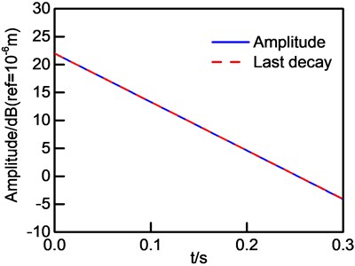
Take a frequency band with two modes as an example, modal parameters are shown in Table 1, where $m$ is modal mass, $k$, $c$ and $s$ represent modal stiffness, modal loss factor coefficient and spectral density of force, respectively. Decay vibration signal of frequency band is shown in Fig. 1, and Fig. 2 illustrates the logarithm of vibration amplitude and initial decay. Loss factor calculated by PIM and IDRM can be checked in Table 2 where error is defined as:

Fig. 1Vibration decay curve

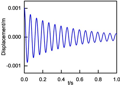
Fig. 2Logarithm of vibration amplitude and initial decay curve

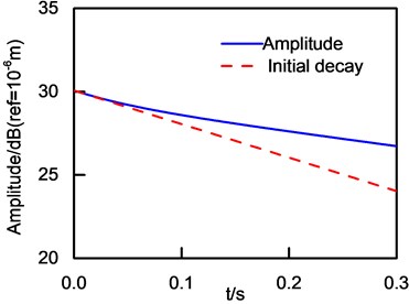
As shown in Table 2, frequency-band loss factor obtained by PIM and IDRM are 5.33×10^-2 and 9.22×10^-2, respectively. It is obvious that frequency-band loss factor from PIM and IDRM are different and the error is nonnegligible. Furthermore, the error will be discussed in detail in Section 5.

3. Frequency-band loss factor estimated by PIM

SEA concerns about frequency-band loss factor which are related to the energy dissipation of structures in frequency band. Loss factors of SEA are ratio of dissipated energy and mechanical energy of structure in a vibrational period [19]. The input power of structure can be calculated by summing the modal input powers and vibration energy summing the modal energies. Therefore, frequency-band loss factor ${\eta }_c$ can be solved by energy balance equation and expressed as:

where ${\omega }_c$ is central angular frequency of frequency band of interests, $f_c$ and$f_i$ denote central frequency of the frequency band and natural frequency, $P_{in}$ is input power of structure, $E$ and $E_i$ represent the vibration energy of structure and modal vibration energy, what’s more, ${\omega }_i$, ${\eta }_i$ and $N$ are the modal angular frequency, modal loss factor, and number of modes, respectively.

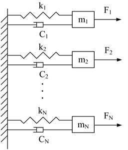
Since the coupling stiffness and coupling loss factors among modes can hardly affect frequency-band loss factor [20], $N$-mode vibration system is able to be simplified as Fig. 3. Equation of motion can be expressed as Eq. (3):

where $x_i$, ${\dot{x}}_i$ and ${\ddot{x}}_i$ are displacement, velocity and acceleration of oscillator, respectively.

Fig. 3Simplified multi-mode vibration system

Assuming external force $F_i$ with spectral density $s_i$ is independent and zero average value in terms of statistics. Thus, complex frequency response function of each oscillator $H_i\left(\omega \right)$ can be formulated as Eq. (4):

The time average displacements and velocities can be expressed as:

It has been proved [2] that the response of resonant zone contributes the most for random forced vibration of oscillator system and:

Modal amplitude of steady vibration can be expressed as:

Assume that $m_i=$1, ($i=$1, 2,…, $N$), Eq. (9) can be obtained:

Substituting Eqs. (4)-(9) to Eq. (2), the frequency-band loss factor can be expressed as Eq. (10):

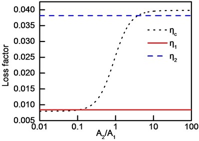
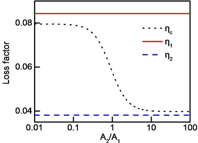
where $R_{sj}=A_j^2/\sum A_i^2$. Take a frequency band with two modes as an example to analyze the effect of vibration amplitude ratio on frequency-band loss factor. There are four cases according to position of the two natural frequencies related to the central frequency: (1) one natural frequency is higher and the other is lower than central frequency. Meanwhile, modal loss factor of higher natural frequency is larger than that of lower natural frequency. (2) One natural frequency is higher and the other is lower than central frequency. Modal loss factor of higher natural frequency is smaller than that of lower natural frequency. (3) Both natural frequencies are lower than central frequency. (4) Both natural frequencies are higher than central frequency. Modal parameters of the four cases and all the modal loss factors and frequencies are shown in Table 3 and Table 4, respectively. Frequency-band loss factors of the four cases are shown in Fig. 4.

As shown in Fig. 4(a), if modal amplitude ratio exceeds a threshold, frequency-band loss factor does not range among all the modal loss factors. What’s more, several conclusions can be obtained as follows: (1) frequency-band loss factor is smaller than all modal loss factors if $A_2/A_1\ll \text{1}$. (2) Frequency-band loss factor is larger than all modal loss factors if $A_2/A_1\gg \text{1.}$ (3) Frequency-band loss factor is between modal loss factors when the two modal amplitudes match each other. It can be explained as follows, respectively: (1) contribution of mode one is far more than that of mode two if $A_2/A_1\ll \text{1}$, which means frequency-band loss factor can be calculated according to modal loss factor at mode one. Meanwhile, natural frequency of mode one is lower than the central frequency so that loss factor of the frequency band is smaller than modal loss factor of mode one. (2) Based on the same procedure as presented previously, the second conclusion is able to be analyzed if $A_2/A_1\gg \text{1}$. (3) Loss factor is affected by both modal loss factor as long as modal amplitude $A_1$ is close to $A_2$. Coefficient of each modal loss factor ranges from 0 to 1 which makes frequency-band loss factor locate between the two modal loss factor.

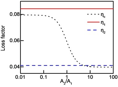
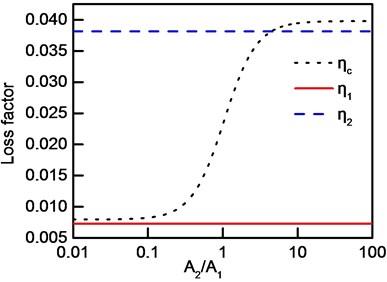
Frequency-band loss factor ranges between modal loss factor over ratio of modal amplitude if one natural frequency, whose modal loss factor is smaller, is higher than the central frequency and the other natural frequency is lower than the central frequency, as shown in Fig. 4(b). According to Fig. 4(c), in the case that both natural frequencies are lower than the central frequency, frequency-band loss factor is smaller than all of the modal loss factors if it is mostly contributed by the smaller modal loss factor, or it ranges between modal loss factors. Furthermore, it can be observed in Fig. 4(d) that both natural frequencies are higher than the central frequency, frequency-band loss factor is larger than all of the modal loss factors if it is mostly contributed by the larger modal loss factor, or it ranges between modal loss factor.

After further analysis of Fig. 4, a conclusion can be obtained that frequency-band loss factor ranges among modal loss factors only if the following condition is satisfied: the modal frequency, whose value of $f_i{\eta }_i$ is the smallest, is higher than central frequency of the band, and the frequency, whose value of $f_i{\eta }_i$ is the largest, is lower than the central frequency.

Fig. 4Frequency-band loss factor: a) case 1, b) case 2, c) case 3, d) case 4

a)

b)

c)

d)

4. Frequency-band loss factor obtained by IDRM

In this section, process loss factor is introduced to describe frequency-band loss factor during decay process, and the way to calculate process loss factor using modal loss factors and modal amplitude is also presented.

For a frequency band with $N$ modes, equation of motion right after the steady excitations are interrupted after steady excitations and it can be expressed as:

where $A_i$ is modal displacement amplitude at initial moment of decay process, and it’s the same as steady displacement amplitude. $A_i$ is able to represent velocity and acceleration amplitude, also. for instance, displacement amplitude will be taken into account as an example to discuss frequency-band loss factor obtained by IDRM.

Assume that displacement of decay process can be written as:

where $A=\sum _{i=1}^N{A}_i$, and ${\eta }_{cp}$ is process loss factor. Substituting Eq. (12) into Eq. (11), process loss factor can be expressed as:

where $R_{pi}=A_i/\sum A_i$. It’s obvious that process loss factor is related to each modal loss factor, modal displacement and time.

Frequency-band loss factor obtained by IDRM is process loss factor when the time equals zero, which is:

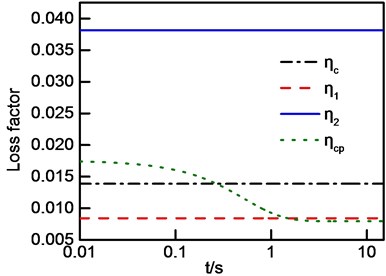
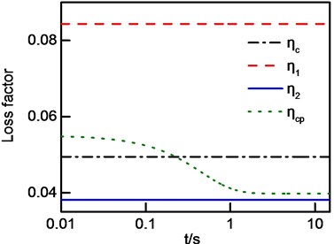
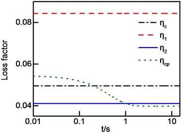
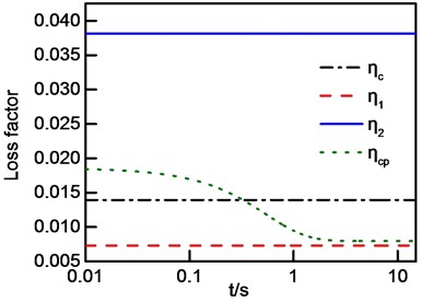
Considering a frequency band with two modes as an example to analyze effect of modal vibration amplitude and time moment of calculation on process loss factor. The modal parameters are the same as Table 5, and the spectral density of excitations are $s_1=\mathrm{}$0.8 and $s_2=\mathrm{}$1. The decay displacement of case 1 is shown in Fig. 5. Process loss factor of four cases are shown in Fig. 6.

As shown in Fig. 6, there is a significant difference between frequency-band loss factor and initial value of process loss factor which is also loss factor of IDRM, thus, there are systematic errors for the estimation of frequency averaged loss factor by using IDRM. Meanwhile, frequency-band loss factor does not change over time, while process loss factor is related to the calculation time moment. Process loss factor tends to frequency-band loss factor contributed by the smallest modal loss factor with time going. This is due to modal displacement of larger modal loss factor decays faster so that modal displacement of mode with larger modal loss factor decreases rapidly comparing with that of mode with smaller modal loss factor. The reason why process loss factor ‘going through’ modal loss factor is that modal frequencies are not equal to central frequency of the band.

Fig. 5Time decay displacement of case 1

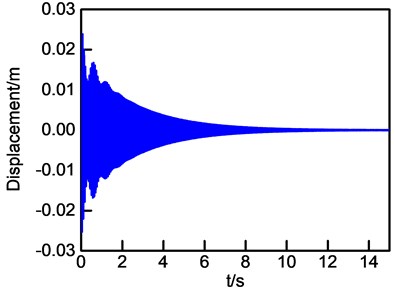
Fig. 6Process Loss factor: a) case 1; b) case 2; c) case 3; d) case 4

a)

b)

c)

d)

5. Systematic error of loss factor obtained by IDRM

Take a frequency band with two modes as an example to analyze error of frequency-band loss factor according to PIM and IDRM. Eq. (10) and Eq. (14) can be reformulated as:

where $n_r=f_2{\eta }_2/f_1{\eta }_1$.

In order to compare the contributions of each mode to frequency-band loss factor obtained by PIM and IDRM, two parameters are defined as:

where $a_r=A_2/A_1$ is modal displacement amplitude ratio. The curves of $R_1$ and $R_2$ are shown in Fig. 7.

Fig. 7The curves of R1 and R2

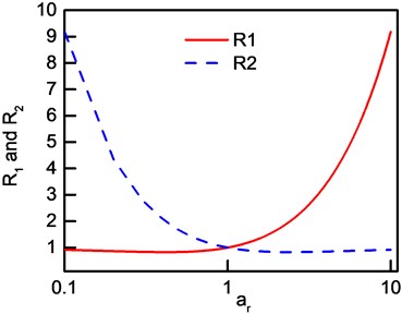
In Fig. 7, it can be observed that both $R_1$ and $R_2$ descend and then ascend simultaneously with the increasing of $a_r$. Further more, it is clear that $R_1$ tends to infinite while $R_2$ tends to 1 with the increasing of $a_r$, and $R_1$ tends to 1 while $R_2$ tends to infinite as $a_r$ approaching infinite. Which means that the error by IDRM is mostly contributed by items related to $R_1$, which are $R_{s1}/n_r$ and $R_{p1}/n_r$. The error decreases with increased $n_r$. The error increases with the increasing of $n_r$ as long as $R_2$ approaching infinite which can be expressed as:

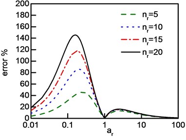
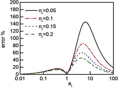
Fig. 8System error of IDRM: a) nr>1, b) nr<1

a)

b)

The errors related to the varying of $n_r$ and $a_r$ is shown in Fig. 8, it can be observed that, the error is zero only if $a_r$ equals one which represents the value of modal amplitudes are the same. In both situations of $a_r>\text{1}$ and $a_r<\text{1}$, the error increases firstly and then descending with the increasing of $a_r$. Additionally, two peaks of errors exist as the increasing of modal amplitude ratio, one of them increases rapidly with increased disparity of modal loss factors while the other is hardly affected by the disparity.

6. Last decay rate separation method (LDRSM)

Modal displacement amplitudes and the multiplication of natural frequencies and related modal loss factors are needed to calculate frequency-band loss factor. Since process loss factor tends to frequency-band loss factor contributed by the smallest modal loss factor, last decay rate separation method, which obtains vibration amplitude and $f_i{\eta }_i$ step by step in the time domain, is proposed to estimate frequency-band loss factor.

For a frequency band with $N$ modes, vibration amplitude can be written with the smallest modal loss factor, related natural frequency and amplitude as Eq. (20) if decay time is long enough:

where ${\eta }_k^{\mathrm{\text{'}}}=\underset{t\to \mathrm{\infty }}{\mathrm{l}\mathrm{i}\mathrm{m}}{\eta }_{cp}=\mathrm{m}\mathrm{i}\mathrm{n}\left({\eta }_i\right)$, $i=\mathrm{}$1, 2,…, $N$, $A_k^{\mathrm{\text{'}}}$ and $f_k^{\mathrm{\text{'}}}$ denote the smallest modal loss factor, related vibration amplitude, and related natural frequency, respectively.

The natural logarithm of vibration amplitude is:

where $S_k=-\pi f_k^{\mathrm{\text{'}}}{\eta }_k^{\mathrm{\text{'}}}$. It can be noticed from in Eq. (21) that a line with slope $S_k$ can be obtained. Meanwhile, $A_k^{\mathrm{\text{'}}}$ is able to be determined by initial value of the line and frequency-band loss factor can be evaluated as Eq. (22) as long as $S_k$ and $A_k^{\mathrm{\text{'}}}$ are obtained:

The process to obtain frequency-band loss factor by using LDRSM are listed as follows:

(1) Get the natural logarithm of tested vibration signal $u_1$.

(2) Calculate $S_k^{\mathrm{\text{'}}}$ according to last decay curve $u_1$, and $A_k^{\mathrm{\text{'}}}$ according to the point of intersection between last decay curve and longitudinal coordinates.

(3) Get a new $u_1$ by eliminating the modal component in step (2) from $u_1$, as shown in Eq. (23).

(4) Repeat step (2) and (3) for $u_1$ to get all $\left\{S_k^{\mathrm{\text{'}}}\right\}$ and $\left\{A_k^{\mathrm{\text{'}}}\right\}$:

where $u_1^{\left(i\right)}$ is $i$th generation of $u_1$.

7. Simulation results

As presented in Section 2, a frequency band with two modes will be discussed in this part. It is easy to calculate natural frequencies $f_1=\mathrm{}$15.1 Hz and $f_2=\mathrm{}$16.7 Hz, modal loss factor ${\eta }_1=\mathrm{}$3.81×10^-1 and ${\eta }_2=\mathrm{}$4.22×10^-2, modal displacement amplitudes $A_1=\mathrm{}$1.58×10^-4 m and $A_2=\mathrm{}$8.58×10^-4 m, and logarithm of vibration amplitude and its last decay are shown in Fig. 9.

$S_1^{\mathrm{\text{'}}}=$–2 according to last decay slope, and $A_1^{\mathrm{\text{'}}}=\mathrm{}$8.58×10^-4 m by using initial value of last decay curve, furthermore $u_1$ can be recalculated by using Eq. (23) and as shown in Fig. 10, and $S_2^{\mathrm{\text{'}}}=\mathrm{}$–20 and $A_2^{\mathrm{\text{'}}}=\mathrm{}$1.58×10^-4 m can also be obtained without any difficulties. Frequency-band loss factor evaluated by IDRM and LDRSM are shown in Table 6.

Fig. 9Logarithm of vibration amplitude and its last decay curve

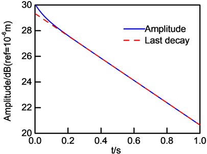
Fig. 10New u1 and its last decay curve

As shown in Table 6, ${\eta }_c$ is frequency-band loss factor identified theoritically by PIM, it corresponds quite well with that obatined by LDRSM, this demonstrates its high accuracy which is able to decrease the error significantly induced by IDRM for the estimation of loss factor.

8. Experimental verification

With the purpose of validating the feasibility and accuracy of proposed method, loss factor experimental test for a steel panel with the dimensions of 0.52 m×0.48 m×0.002 m was carried out. The experimental system is shown in Fig. 11, in which one edge of the panel was hanging on to simulate free boundary condition and white noise signal is applied to excite the whole structure at the corner.

Fig. 11Experimental system

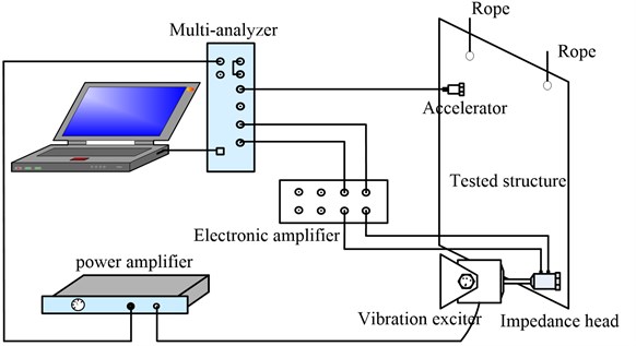
From Fig. 12, it can be seen that the panel was divided into nine zones, exciting point is in the ninth zone, and each zone is bonded with a sensor where the average measurements of these transducers is considered as the final output signal. Data of PIM was recorded in 1/3 octave, and the input power was tested by cross spectrum of force and velocity for the driving point and energy by averaging energies of the nine zones. Loss factor obtained by PIM can be calculated from the input power and energy. Meanwhile, data of LDRSM and IDRM was recorded in time domain as long as the exciter was turned off from the steady vibration state. Finally, loss factors obtained by LDRSM and IDRM are the averaged values resulting from nine subsections.

Fig. 12Divided zones of the panel

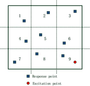
Fig. 13Absolute value of displacement

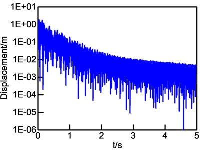
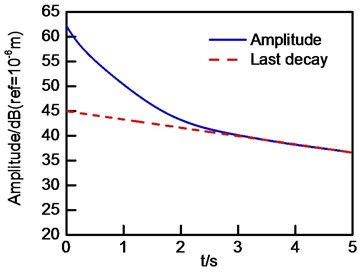
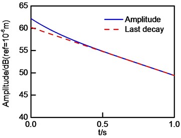
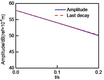
Fig. 14The evolutionary of u1and its related last decay curves: a) u1 and its last decay curve in initial generation; b) u1 and its last decay curve in first generation; c) u1 and its last decay curve in second generation

a)

b)

c)

To describe the procedure of proposed method, 200 Hz was predefined as central frequency and the absolute displacement is shown in Fig. 13. $u_1$ and related last decay curves and loss factor evaluated by the three strategies are illustrated in Fig. 14 and Table 7, respectively. Frequency-band loss factor based on PIM is considered as theoretical value, and it is clear that LDRSM is more accurate than IDRM comparing the errors of IDRM and LDRSM which calculated by Eq. (1) as shown in Table 7.

9. Conclusions

Research on estimation of frequency-band loss factor with multi-modes has been conducted. The following conclusions are drawn from the results of the study.

1) Frequency-band loss factor is not always among modal loss factors but related to contributions of vibrational amplitudes and modal loss factors.

2) Frequency-band loss factor ranges among modal loss factor only if the following two conditions are satisfied simultaneously: a) the modal frequency, whose value of $f_i{\eta }_i$ is the smallest, is higher than central frequency of the band, b) the frequency, whose value of $f_i{\eta }_i$ is the largest, is lower than the central frequency.

3) Process loss factor, which is related to each modal loss factor, modal displacement and time, has been introduced in such a way that it has the same value as frequency-band loss factor obtained by IDRM at the initial moment of decay. However, it tends to frequency-band loss factor due to the contribution from smallest modal loss factor with time going.

4) LDRSM has been implemented to evaluate frequency-band loss factor. In comparison of experimental results, it is demonstrated that LDRSM has a higher accuracy than IDRM whose errors can be reduced significantly with satisfied fidelity.