Abstract
The artillery weapon system muzzle disturbance is influenced largely by the carrier vibration through firing. In case of military trucks carrying cannons, the longitudinal bending vibration is the most important factor affects the muzzle disturbance. The corner stone of this article is the modal and sensitivity analysis of a chosen military truck carrying cannon in order to investigate how much the longitudinal bending natural frequencies of this truck deviated from the nominal value as a result of truck components layout or position variation and some system design parameters variations. This deviation is examined to clarify the most sensitive parameters that affect the longitudinal bending natural frequency. The dynamic characteristics of the truck, such as the natural frequencies and the mode shapes, are determined by using finite element method in order to create the truck flexible system. Via intermediate file, the flexible truck model is imported into commercial FE code “ABAQUS” software for modal analysis whose solutions agree well with an experimental data. This study shows a complete and deep investigation of the dynamic response calculations for a complex flexible military truck. In addition, the sensitivity analysis compels the designer to identify the critical variables which affect the longitudinal bending vibration beside obtain additional information about weapon system dynamics.
1. Introduction
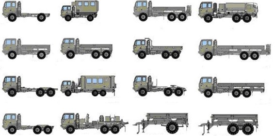
Trucks vary greatly in size, power, and configurations. Nevertheless, they share many common constructions like chassis, driver cabinet, axles, suspensions, road wheels, engine, and a drive-train beside many associated systems as Pneumatic, Hydraulic, Water, and Electrical systems as shown in Fig. 1. The Military Trucks (MT) have many added parts comparing with the civilian one such as tilting legs, gun housing, gun frame, ammunition housing, bombardment, mine detonation, etc.
Fig. 1Different samples types of military truck families
Usually, the guns system are trailed by trucks and not loaded on them but in case of loading guns on trucks, tracked vehicles are used to install the gun components. Therefore, most studies in the truck dynamics have focused on the vibration of the truck structure system without gun components, while other articles and studies in the gun dynamics have concerned in the gun vibration without carrier structure system. Very few studies are interested in the dynamic behavior of the whole system for both truck and gun components especially for this family of weapons systems. At most, these studies interested in determining the minimum Natural Frequencies (NF) for the whole truck structure system through calculations by FE software’s packages or by process real measurements. But the study of Longitudinal Bending (LB) NF variation against different Design Variables (DV) is not most likely considerable. Therefore, here in this article, the studying of whole truck system dynamics is as important to be examined and tested.
By virtue of the MT works in the battle field, it must be more rigid and more reliable comparing with the civilian one. Of course, the weight must be at the slightest degree to grantee the mobility. All MT tasks are greatly influenced by the system vibration behavior. The most effective part in the truck vibration is the main chassis [1, 2]. Taking in Consideration the nature of the relationship between the truck chassis length and width beside the masses distribution around the truck chassis [3], it is clear that truck chassis always vibrates in LB direction. Unfortunately this LB vibration affects strongly many tasks of the MT. For example and not as a limitation, the firing accuracy and density focused by Muzzle Disturbance (MD) are greatly affected by this type of vibration behavior in addition to a decrease in the truck working age because of the weakness of some parts and connections as a result of vibration. The vibration behavior of the MT, through attacking maneuver or fighting, is highly dependent on the NF or resonant frequencies and mode shapes of the carrier system. More often, the only desired modes are the lowest frequencies especially in the LB because they can be the most prominent modes at which the trucks will vibrate.
Finite Element Model (FEM) is generated for a chosen truck caring cannon in order to investigate completely the dynamic performance. To grantee the accuracy of the truck system FEM, it’s important to define carefully the connection between different components. Unfortunately, the FEM numerical results for a single part is quite accurate and reliable in both theory and application, while the connection modeling between components in complex structure is still far away from the real situation. The most important question, when studying the NF of a complex structure system consists of different components with different thickness and different 3 dimension model shapes, is how to generate the FE model of these parts and what is the nature of the connection between them to grantee accuracy and to reflect the real world. Mostly, the connections simulation between different components of complex structure systems in FEM is rigid which is not in conformity with the reality. Also, the Boundary Conditions (BC) should be defined precisely because it has a great impact on the FEM numerical results. To match the FEM numerical result with the experiment results, different types of connections between truck components are created and tested. In addition, the effect of truck layout variation, soil types, and the suspension system stiffness variations on the FEM numerical results are also examined and tested. Also, the BC of the FEM are changed to investigate the effect of BC changing on the truck minimum NF variations.
This study especially the sensitivity analysis will help in future to increase the design robustness of this type of weapon system. In addition, it assists the designer to examine the possibility of incorporating a hydraulic control circuit to the weapon system in order to decrease the system vibration through firing mode, whereas the sensitivity analysis will represent the critical parameters that affect the LB vibration. It is planed that this hydraulic control circuit will consist of two hydraulic cylinders instead of the left and right instillation legs which will be controlled via non-linear controller.
2. Truck vibration and structure system composition
The Mechanical vibrations in trucks occur as a result of continuous transformation of Kinetic Energy to potential Energy, back and forth. Common reasons of the civilian trucks vibration are poor wheel balance, imperfect tire or wheel shape, brake pulsation, and worn or loose driveline, suspension, or steering components [4]. In case of MT, in addition to these reasons, some detrimental vibrations as a result of structural parts flexibility under firing conditions are added to the system vibration reasons. Flexibility of structures components such as frames, connections, housing, tires axis and suspension links can also contribute to springing, especially to damping out high frequency vibrations. However, due to weight, maneuverability and cost requirements, the truck structures are not been more rigid than necessary. In MT, the flexibility is mainly in the chassis part, ammunition reloads system, and gun or gun housing if exists. Fig. 2(a), represents the virtual image of the whole weapon system case of study contains the cannon barrel, gun reload system, firing control system, ammunitions reloads system and three installing feet. While, geometrical 3D model of the actual MT carrier case of study created by “CREO/PARAMETRIC 2.0” is presented in Fig. 2(b). This MT, on detailed explanation, consists of chassis, driving room, front and back engine blocks, tiers and tires axis, suspension system, gun system, front and back ammunition reloads system, installation legs, fuel tank, oil tank, and firing control system. Due the complicated structure of the gun system, ammunition reload systems, suspension system, and firing control system, the detailed 3 dimensional model of them is shoved overlooked in details.
Fig. 2Artillery weapon system case of study: a) virtual image of the whole weapon system; b) 3D model of the carrier military truck including selected frame of reference

a)
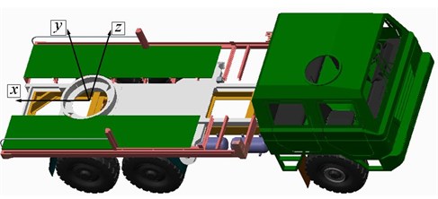
b)
3. Free vibration analysis fundamentals
This section briefly describes some of the numerical methods used in finite element analysis for solving eigenvalue problem of a free vibrated structure, while fuller details may be found in the references [5-11]. In order to determine the frequencies, and modes, of a free vibration structure, it is necessary to solve the linear eigenvalue problem presented in Eq. (1), where and are the stiffness and inertia matrices respectively:
Whichever method is used to calculate the eigenvalues and eigenvectors, it is useful to be able to determine the number of eigenvalues in a specified range. This is a useful piece of information when designing a structure against vibration. In addition, this information can be used to check that the method used has located all the eigenvalues. Also, the number of eigenvalues less than a specified value of can be determined using a Sturm Sequence method [5]. This method can be simply applied by substituting the values of , , and in Eq. (2):
There are different methods used to calculate and solve the eigenvalue problem. One of the most famous methods is the Jacobi method which is based on applying a sequence of orthogonal transformations in the form presented in Eq. (3). Each transformation eliminates one pair of off-diagonal elements of a symmetric matrix:
One problem with this method is that the search for the largest element is time consuming. This can be overcome by using the cyclic Jacobi procedure. In addition, the disadvantage is that regardless of its size, an off-diagonal element is always zeroed. A more effective procedure is the threshold Jacobi method. Instead of eliminating all the elements in the cyclic method, those having a modulus below a given threshold value are left unaltered. When all of the elements have a modulus below the threshold value, the threshold value is reduced and the process repeated. Iteration is complete when the threshold value has been reduced to the required tolerance.
The other famous procedure is Givens’ and Householder’s methods. This method based on reduces the matrix [] to tri-diagonal form using a finite number of transformations. The eigenvalues and eigenvectors of the tri-diagonal matrix have then to be determined by a separate technique. This method is combination between two methods. The Givens method which uses the Jacobi transformation to reduce element (1, ) to zero rather than element (, ). The Householder method uses a sequence of orthogonal transformations, each one of which produces a complete row and column of zeros apart from the elements within the tri-diagonal form.
The other method is bisection which is described for determining the eigenvalues of a symmetric tri-diagonal matrix. The eigenvectors are obtained using inverse iteration where the first step in the bisection method is to determine upper and lower bounds for all the eigenvalues. One of the simplest methods for determining such bounds is by Gershgorin which is presented in Eqs. (4), (5):
Finally, the LR, QR and QL methods are also have many applications in eigenvalue problem calculations. The LR, QR and QL methods all use a sequence of similarity transformations to transform the matrix A to either upper or lower triangular form. The eigenvalues of such a matrix are then equal to the elements on the main diagonal. The methods can be applied to a fully populated matrix, but it has been found in practice that it is more efficient to reduce the matrix to tri-diagonal form, using either Givens’ or Householder’s method, before applying one of these techniques. Each method will produce both eigenvalues and eigenvectors, but in practice too much storage is required to calculate the eigenvectors. It is, therefore, usual to determine only the eigenvalues and then use the method of inverse iteration to calculate the eigenvectors.
4. Dynamic analysis fundamentals of FEM by using ABAQUS
ABAQUS is one of the most popular programs in the FE analysis use implicit integration scheme and, in addition, to explicit special purpose FE analyzer. ABAQUS/AMS, the automatic multi-level substructuring eigensolver, is used to compute the eigensolution for the FEM. A steady-state dynamic analysis is then performed in ABAQUS/Standard [12]. The ABAQUS eigensolver version 6.13 is used to calculate the dynamic analysis for the case study of MT in this article. Dynamic modeling in ABAQUS is very easy and can provide very meaningful results. As any package of FE program the FE analysis in ABAQUS consists of 3 separate stages. These stages are pre-processing, processing, and post-processing. The first stage is normally more difficult, because the complexity of the components shapes. In the second stage the basic equations of continuum mechanics in both cases of kinetics and kinematics are formulated to build a complete FE problem. The fundamental relations of continuum mechanics are based on the local basic balance equations. The continuity equation, in case of conserved mass, is one of these balance equations and can be expressed in Eq. (6):
The balance of linear and angular momentum is the second balance equation and can be expressed in Eq. (7):
Also, the first law of thermodynamics is an important law in the fundamental relations of continuum mechanics and can be expressed in Eq. (8). Finally the strong form of the EOM for FEM is presented in Eq. (9):
where is the symmetric Cauchy stress tensor, the density, the body forces and the velocity. The kinematical relations and balance laws are not sufficient to solve a boundary or initial value problem in continuum mechanics. For a complete set of equations, a constitutive equation has to be formulated which characterizes the material response of a solid body like strain. Simply, strain is the change in the body lengths that occurs as the body deforms from the initial to the current configuration. Several approaches can be used to transform the physical formulation of the problem to its FE discrete analogue as mentioned before. If the physical formulation of the problem is known as a differential equation then the most popular method of its FE formulation is the Galerkin method. If the physical problem can be formulated as minimization of a functional then variational formulation of the FE equations is usually used.
5. Finite element modeling of a complex military truck structure case of study
5.1. Assumptions
When building the FEM of this complex truck system, are taken in consideration as follow:
1) The fixation of this truck through firing is based mainly on the three installation legs. While in fact, the fixation on the truck tire is neglected in the stability calculations. This leads to assume the deformation on the tire is very small in order to be assumed linear elastic range. Then the material definitions of the tires elements will be linear elastic material obey hooks low [13-15].
2) All parts are linear elastic bodies obey hooks low [16] except the tire which is in fact considered as a viscoelastic body. Also, the assembly gaps between parts are neglected.
3) In some cases the connections between different weapon system components are rigid through FEM nodes. In other cases that allow linking two different extended surfaces by certain material slice, a matching thickness material slice are synthesized to serve as a simulation of the welding between these two surfaces.
4) As a result of the unnecessary tiers axis meshing studies, and huge axis configuration irregularities, the FEM is generated for the three tires axis as beam section with constant diameter circular cross-section.
5) Due to the extreme complexity of front and rear ammunition reload system, and firing control system besides the unneeded building FEM for those parts in details, a simplified FEM is generated. Nevertheless, the masses and inertia tensor are guaranteed for those parts. Also, fuel and oil tanks, rear and front engines, and rear instillation leg components are added as point mass and inertia tensor matched with the real data in ABAQUS program. The propellant charge and the bullet are neglected in FEM.
6) In order to facilitate the FE Modal Analysis (MA) of the truck system, gun components FEM of appropriate simplification are generated. This FEM is produced to keep the main real features of the gun system in addition to the masses and the inertia of whole gun system. The same way is applied to generate the FEM of the driver room but with more simplification. There are some parts in the driver cabinet machines are omitted in FEM like motor, control wheel, door details etc., which are not affecting the modal analysis of the truck assembly.
5.2. Global coordinate system and units
The origin of the global coordinate system is the traverse center of the gun as shown in Figs. 2 and 3. The global -axis is the horizontal axis passes through the main longitudinal truck axis and from the driver cabinet to the firing point, the global -axis is the vertical line against gravity, and the global -axis satisfies right hand rule. Also, The SI system of units is used throughout this paper.
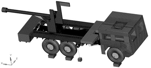
Fig. 3FEM for the whole military truck components case of under study
5.3. Finite element model
In order to guarantee accuracy and reliability, professional meshing software HYPERMESH is applied to build the FEM of the complex structure truck system. Different types of elements are used in the model, 1-D, 2-D, 3-D, wedgy, beam, spring, in addition to rigid elements as shown in Figs. 3-5. Also some components are added as point masses with inertia tensors like fuel and oil tank as mentioned in the assumptions. The rigid elements are used to connect some parts like tires with the tires axis to simulate the non-involved study connections. The materials that have been defined for the whole FEM are basically steel with normal properties beside some needed material have been defined so that the FEM results become closer to the reality like the 6 tires which the material that defined is rubber. This closeness in materials definitions leads the FEM results match with the experimental results. The constructed FEM consists of 330285 nods, 360475 elements, and 1978236 D.O.F, 10 assemblies, 63 components, 39 properties for different shell thickness, and 15 types of materials. The definition of the modulus of elasticity of the truck components materials, Poisson’s ratio, and material density uses the following units: Length [mm], mass [Ton], density [Ton/mm3], force [N], stress [MPa], spring stiffness [1e-3 N/m] angle [Degree], and time [s]. The mass of the whole system is about 16.5 Tons included gun and ammunition blocks.
5.4. Boundary condition
This truck is tilting up on three feet to ensure stability and equilibrium through firing in combat. Also, sometimes the tires touch the ground to keep the friction between the truck and the soil through firing in the maximum level. But due to the highest flexibility level and the viscoelastic property of tiers, sometimes this interaction between tiers and soil can increase the vibration through firing and decrease the accuracy. Therefore the tire and soil interactions are neglected in stability calculation as mentioned before. This means that the BC for this type of truck are not fixed for all cases. For example, the truck can be installed on the 3 legs only or by adding a contact friction between tires and soil. Hence, the importance of the study for the various types of BC effect on the NF variation becomes obvious. Four types of BC are selected and listed with their abbreviation in Table 1 for this MA simulation.
Fig. 4FEM of the military truck lower chassis, installation legs holders, simulated ground piece
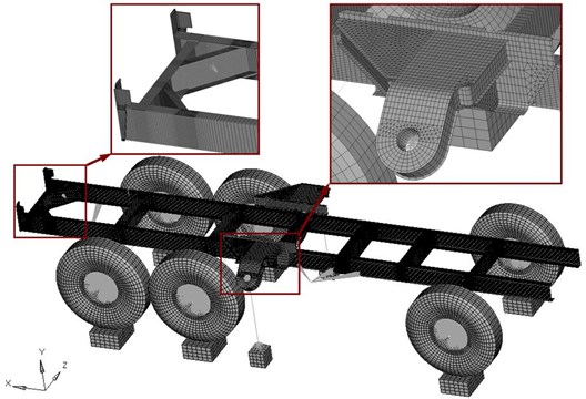
Fig. 5FEM of the military truck upper carriage, gun housing, rear ammunition, and front
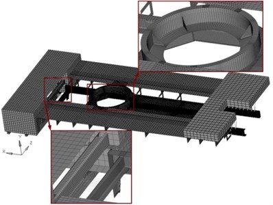
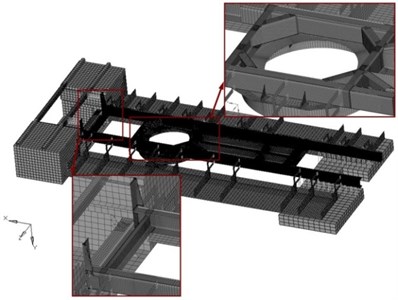
Table 1Different cases boundary conditions definition
BC abbreviation | BC definitions |
9P | 6 tires touch the ground beside 3 instillation legs |
5P | Just front tires touch the ground beside 3 instillation legs |
3P | 3 instillation legs are carried out the whole truck structure without any other contact between truck components and soil |
NP | Without any contact where ABAQUS program can implement the simulation calculations without any BC as if the truck hovers in a vacuum without presence of the |
There are several studies to calculate the stiffness value that simulate the soil interaction with tires or with steel plate like here in the instillation legs [17, 18]. Also the tire stiffness value can be deduced by many ways. But in this case all of these studies are neglected because this is not the scope of the article. The most significant problem in modeling of the BC in this FEM is the modeling of the tires and the contact between tires and different types of soils because mostly the calculated NF belongs to the tires in different mode shapes not the whole system. This is normal because the tiers are more flexible than the other parts of the FEM model. To avoid this problem, different BC with different values and different tiers properties are created and tested until the simulation results match the experiment results. In the case of contact position between the three instillation legs and the soil, three complete fixations BC are applied. In addition, 6 spring connections are generated between the tires axis and truck lower chassis to simulate the suspensions system of the truck.
6. Modal analysis
6.1. Modal analysis numerical results of the case under study
The MA is computed in ABAQUS software for the whole truck structure system at different BC listed in Table 1. Table 2 represents the values for some DV in this FEM. The values of suspension stiffness presented in Table 3 are chosen to achieve outcomes near to the experimental results and to reflect as possible the suspension values in the real world.
Table 2Different cases boundary conditions definition
Spring | N/mm | Interaction Modulus of elasticity | MPa |
Front suspension | 60 | Soil under tires | 100 |
Middle | 90 | Soil under 3 legs | 6800 |
Rear suspension | 90 | 6 Tiers | 3e4 |
Table 3Truck natural frequency simulation and experimental results at different boundary conditions
Simulation results | Experimental results | Error % | ||||
BC type | LBNF (Hz) | HSNF (Hz) | LBNF (Hz) | HSNF (Hz) | LBNF | HSNF |
9P | 4.77 | 5.47 | 4.65 | 5.31 | 2.7 % | 2.9 % |
5P | 4.77 | 5.46 | 4.65 | 5.31 | ||
3P | 4.01 | 4.84 | ||||
NP | 7.04 | 10.51 | ||||
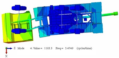
It is well known that the first natural frequency of truck system behaves in a rigid body motion manner. In this weapon type the Longitudinal Bending Natural Frequencies (LBNF) is the dominant motif generated from the carrier system that effects greatly the firing dispersion as a result of firing vibration. So, LBNF is the sensitive parameters need precise investigation comparing with the other NF. The LBNF results obtained from ABAQUS software at different types of BC are presented in Table 3. It’s logical that there are no big difference between FEM results in both 9P and 5P cases because the truck is already fixed on the 3 instillation legs. Also, this outcome confirms the assumption of the tire simulation as a linear elastic material. If all tires don’t touch the ground a small logic decreases in NF must be exist witch is clearly defined in Table 3 this proves the validity of the simulation program results. Fig. 6 lists the first 4 mode shapes results obtained from “ABAQUS” software under the first type of BC in addition to 6 springs with stiffness presented in Table 2 connected between the 3 tires axis and the truck chassis. Also, these mode shapes of these frequencies are depicted in the same figure. To verify the FEM calculated results, it is necessary to implement the practical test to calculate the first NF. The details of this test are not different in nature from normal modal analysis tests beside that the LBNF is the dominant parameters needed to be studied. Therefore, the experiment details are omitted here to avoid dispersion in the article focus. The experimental test numerical results confirm that the first NF at the first and second types of the BC is the LBNF in case of neglecting the rigid body motion manner with value 4.65 Hz. Also, the second NF at the first and second type of BC is the Horizontal Shear Natural Frequencies (HSNF) with value 5.31 Hz. This means that the FEM just has around 2.7 % error in the first mode, and 2.9 % error in the second mode comparing with the experimental results. Of course this convergence between measurements and FEM results confirms the validity and accuracy of the FEM created for this type of truck.
Some conclusions are drawn as follows from the results.
1) Mass of the FEM is a little larger than that of the real system which can cause error in the numerical results. Also, the welding simulation in FEM model may be more rigid than the reality which make the model slightly more rigid and cause this little upper shift in the numerical result.
2) The first effective vibration mode shape is the longitudinal bending in the truck chassis which reflect the reality. This result is logic because of the long length of the vehicle, about 8 meters, without barrel in addition to the mass nature distribution along truck length. Errors in the first and the second mode shapes are in an acceptable range.
3) The Decrease in the simulation results of the HSNF due to change the type of BC from 9P or 5P to 3P is a logical result. This is because the usage of vehicle tires increases the body’s resistance to the curvature in the transverse direction
4) The second and third vibration mode shape is the vibration of the 6 tires which is very near to the value of the first mode. These vibration modes are neglected due to the improper uses.
5) The fourth vibration mode is horizontal shear for the weakest position of the truck chassis. This weak position is quite clear in the bottom view.
6) The next resulted mode is rolling mode, while the last resulted mode is complete vibration for the whole truck components.
7) There are many DV affect the numerical results like suspension stiffness, truck layout, contact type between soil and truck etc. need to be studied for complete investigation of the FEM vibration behavior.
Fig. 6Truck mode shapes at 9P BC: a) mode 1 longitudinal bending ωn= 4.7 Hz; b) mode 2 horizontal shear ωn= 5.5 Hz; c) mode 3 horizontal torsion ωn= 11 Hz; d) mode 4 ωn= 13.8 Hz
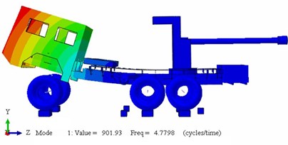
a)
b)
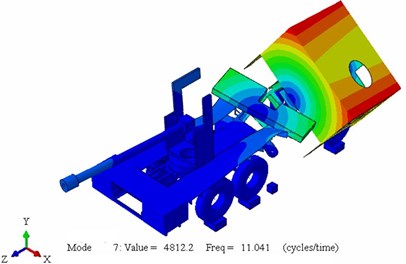
c)
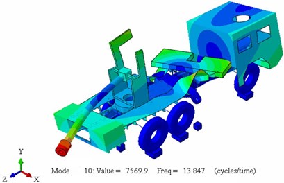
d)
6.2. Design variable sensitivity
As mentioned before the most important vibration behavior in the MT is the LB vibration which is the most significant vibration generated form vibration of the gun carrier affects the firing dispersion. Also it’s mentioned that there are many DV affect this type of vibration mode. These DV are studied separately to investigate their effect on the LBNF value of the truck under study. DV are divided into 2 groups based on 2 fundamental basics studies. The first is components parameters values, like spring stiffness for the suspension system, while the other is based on truck structure components layout, like instillation leg position variation, in order to clarify their effect on the LBNF. The first DV group is presented in Table 4 including the modulus of elasticity for different types of soils that simulate interaction between legs plates and soils. It’s mentioned in the introduction of this article that there are many studies for calculating the modulus of elasticity for a soils piece that contact with tires. It is sufficient in this case to study the effect of the soil through change the value of the modulus of elasticity in order to simulate different types of soils.
By studying Table 4 it’s clear that all these DV don’t have any significant effect on the LBNF vibrations except the modulus of elasticity variation of the soils which is contact with instillation legs. This is of course logical outcomes because in fact the first design variable can’t affect the vibration in the LB direction. The same logic results are presented in the second design variable which the numerical variation of Stiffness value of the gun equilibrator which just affect the vibration behavior of barrel. In the case of modulus of elasticity variation for different types of soils that touch the 6 tires, it also can not affect the LB because of the presence of 3 legs with direct steel contact with soil which is in fact more rigid than tire and soil interaction. These different types of soils modulus of elasticity are presented in Fig. 7. Fig. 7 clearly shows that the modulus of elasticity variation have a significant effect on the LBNF values especially when it decreases to value less than 6 GPa. These numerical results reflect the vibration behavior in the real world, which mean that the interaction between soil and installation legs must be at the maximum level and for these reasons in the reality plates of steel added to the installation legs to keep the interaction elasticity in the maximum level.
Table 4First DV set affects the LBNF variation
DV | DV range | BC type | LBNF Hz | DV | DV range | BC type | LBNF Hz | DV | DV range | BC type | LBNF Hz |
Friction coefficient between soil and tier surfaces | 0.2 | 9P | 4.711 | Stiffness value of the cannon equilibrator between barrel and gun carriage (N/mm) | 5 | 9P | 4.735 | Modulus of elasticity for different types of soils that simulate interaction between legs plates and soils (MPa) | 100 | 3P | 2.78 |
5P | 4.701 | 5P | 4.731 | 200 | 2.9 | ||||||
0.35 | 9P | 4.713 | 15 | 9P | 4.739 | 300 | 2.92 | ||||
5P | 4.705 | 5P | 4.733 | 400 | 3.1 | ||||||
0.5 | 9P | 4.716 | 25 | 9P | 4.742 | 500 | 3.21 | ||||
5P | 4.710 | 5P | 4.735 | 700 | 3.5 | ||||||
0.65 | 9P | 4.716 | 35 | 9P | 4.744 | 1000 | 3.71 | ||||
5P | 4.712 | 5P | 4.739 | 1200 | 3.77 | ||||||
0.8 | 9P | 4.719 | 45 | 9P | 4.746 | 1500 | 3.8 | ||||
5P | 4.712 | 5P | 4.741 | 2000 | 3.85 | ||||||
Modulus of elasticity for different types of soils that touch the 6 tires (Mpa) | 50 | 9P | 4.701 | 65 | 9P | 4.751 | 3000 | 3.88 | |||
5P | 4.692 | 5P | 4.745 | 5500 | 4.1 | ||||||
200 | 9P | 4.698 | 85 | 9P | 4.756 | 6000 | 4.25 | ||||
5P | 4.695 | 5P | 4.751 | 6500 | 4.46 | ||||||
500 | 9P | 4.702 | 105 | 9P | 4.761 | 6900 | 4.67 | ||||
5P | 4.700 | 5P | 4.757 | 7000 | 4.71 | ||||||
1000 | 9P | 4.709 | 125 | 9P | 4.769 | 7500 | 4.78 | ||||
5P | 4.703 | 5P | 4.761 | 10000 | 4.52 | ||||||
5000 | 9P | 4.710 | Complete rigid | 9P | 4.779 | 15000 | 4.31 | ||||
5P | 4.709 | 5P | 4.768 | 30000 | 4.15 |
In the next DV group, different structure layout variation are tested and examined. A gun traverse center is one of important DV variation needs to check its effect on LBNF. Table 4 represents the effect of this position variation in addition to rear, right, and left longitudinal position variation from their original position on the LBNF. Table 4 shows that the gun traverse center position variation doesn’t have quite effect on the LBNF. This is because the weight of the gun is not very big comparing with the truck total mass. Also, the position variation is still in the longitudinal axis but if the position variation changes across this axis, the results will completely change. This study is not tested here because it doesn’t reflect the reality that the gun always is assembled in the center of the MT.
As mentioned before, MT always use instillation legs to keep stability during firing in the maximum level in order to insure the firing performance of the gun. Therefore, the effect of longitudinal position variation of these legs on the LBNF is presented in Table 5. By studying the numerical results in Table 5, it’s clear that the rear leg doesn’t have clearly effect on the LBNF comparing with left and right leg. The position variation of left and right instillation legs affect on the LBNF presented in Fig. 7(b).
Table 5Second DV set affects the LBNF variation
DV | DV range | BC type | LBNF Hz | DV | DV range | BC type | LBNF Hz | DV | DV range | BC type | LBNF Hz |
Gun traverse center longitudinal position variation from the original position (mm) | –450 | 9P | 4.72 | Rear leg longitudinal position variation from the original position (mm) | –450 | 9P | 4.75 | Left and right legs longitudinal position variation from the original position (mm) | –450 | 9P | 5.23 |
5P | 4.72 | 5P | 4.75 | 5P | 5.23 | ||||||
3P | 4.01 | 3P | 4.03 | 3P | 4.47 | ||||||
NP | 6.98 | NP | 6.87 | NP | 6.91 | ||||||
–300 | 9P | 4.72 | –300 | 9P | 4.74 | –300 | 9P | 5.06 | |||
5P | 4.72 | 5P | 4.74 | 5P | 5.06 | ||||||
3P | 4.01 | 3P | 4.02 | 3P | 4.32 | ||||||
NP | 6.98 | NP | 6.87 | NP | 6.91 | ||||||
–150 | 9P | 4.71 | –150 | 9P | 4.73 | –150 | 9P | 4.94 | |||
5P | 4.71 | 5P | 4.73 | 5P | 494 | ||||||
3P | 4.00 | 3P | 4.01 | 3P | 4.21 | ||||||
NP | 6.90 | NP | 6.87 | NP | 6.95 | ||||||
150 | 9P | 4.69 | 150 | 9P | 4.69 | 150 | 9P | 4.50 | |||
5P | 4.69 | 5P | 4.69 | 5P | 4.50 | ||||||
3P | 3.99 | 3P | 4.01 | 3P | 3.76 | ||||||
NP | 6.72 | NP | 6.87 | NP | 6.84 | ||||||
300 | 9P | 4.68 | 300 | 9P | 4.68 | 300 | 9P | 4.32 | |||
5P | 4.68 | 5P | 4.68 | 5P | 4.32 | ||||||
3P | 3.99 | 3P | 4.01 | 3P | 3.62 | ||||||
NP | 6.87 | NP | 6.87 | NP | 6.84 | ||||||
450 | 9P | 4.68 | 450 | 9P | 4.66 | 450 | 9P | 4.18 | |||
5P | 4.68 | 5P | 4.66 | 5P | 4.18 | ||||||
3P | 3.98 | 3P | 3.9 | 3P | 3.49 | ||||||
NP | 6.61 | NP | 6.87 | NP | 6.83 |
With a simple studying of Fig. 7(b), the fact of the effect of position variation for left and right instillation legs on the LBNF clearly exists. Also the numerical results difference between the FEM at 9P and 5BC is very small in order to be neglect. The variation of NF variation due to this design variable is about 22 % which is important variation need to be studied and taken in consideration. In case of “NP” the variation of NF is not high because the mass of the left and right legs is about 200 Kg which is about 1.2 % form the whole mass of the truck so they can’t make dominant variation on the LBNF. The longitudinal position variation of the left and right legs can be changed to increase the minimum value NF by about 10 %. The crosswise position variations for the left and right instillation legs are omitted here because this maybe needs another shape or another design for these legs and this is not the scope of this article.
7. Conclusions
Using of FEM method for complete investigation the dynamic performance of the MT is sufficient especially when the numerical results of the FEM are matched with the experimental results which make the results more logic and more acceptable. Chassis in MT must be rigid enough to be able to carry these huge masses and to avoid small or unexpected values for the NF of their structure in order to keep stability of the truck during maneuvering or firing. As a result from sensitivity studies, the NF of the whole structure of the MT is highly depending on the truck layout comparing with other DV like modulus of elasticity variation of the truck tires. The LBNF for this type of MT during standing for firing in case of added tires to fix the truck is about 4.7 Hz, while in case of fixing by only 3 legs, this NF decreases to about 4 Hz. By studying different sets of DV variation effect on the LBNF variation, it is clear now that there are 2 DV have sensitive affection on the variation of LBNF. These deign variables are basically the modulus of elasticity of the interaction between soil and instillation legs, and the instillation legs position variation. The simulated modulus of elasticity for this interaction must be higher than 1500 MPa to avoid rapid decreasing in minimum NF. The longitudinal position variation of the left and right legs can improve the LBNF by about 10 %. Finally, a complete investigation for the dynamic performance of a chosen MT is created in this article.
Fig. 7LBNF variation: a) effect of soil modulus of elasticity variation; b) effect of left and right leg position variation
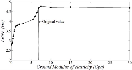
a)
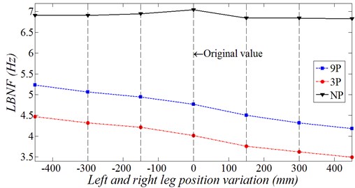
b)
References
-
Novotný P., Píštěk V., Stodola J. Virtual engine-a tool for military truck reliability increase. Journal of Advanced in Military Technology, Vol. 1, 2006, p. 49-70.
-
Novotný P. Cranktrain Dynamics Simulation – Central Module of Virtual Engine. Ph.D. Thesis, Brno University of Technology, 2005
-
Zhong S., Zhao D., Sun Y., Wei Q. Modeling and modal analysis of truck chassis based on FEM. Journal of Machinery Design and Manufacture, Vol. 6, 2008.
-
Jazar N. Vehicle Dynamics. Theory and Applications. Riverdale, Springer Science, New York, 2008.
-
Petyt Maurice Introduction to Finite Element Vibration Analysis. Cambridge University Press, New York, 1990.
-
Wilkinson J. H. The Algebraic Eigenvalue Problem. Clarendon Press, Oxford, 1965.
-
Bishop R. E. D., Gladwell G. M. L., Michaelson S. The Matrix Analysis is of Vibration. Cambridge University Press, New York, 1965.
-
Gourlay A. R., Watson G. A. Computational Methods for Matrix Eigenproblems. Wiley, Chichester, 1973.
-
Bathe K.-J., Wilson E. L. Numerical Methods in Finite Element Analysis. Prentice-Hall, Englewood Cliffs, 1976.
-
Jennings A. Matrix Computation for Engineers and Scientists. Wiley, Chichester, 1977.
-
Bathe Klaus-Jürgen Finite Element Procedure. Prentice Hall, New Jersey, 1996.
-
Hibbitt K. Sorensen ABAQUS: User’s Manual: Version 6.13. Incorporated, 2013.
-
Abeels P. F. J. Tire deflection and contact studies. Journal of Terramechanics, Vol. 13, Issue 3, 1976, p. 183-196.
-
Captain K. M., A. B. Boghani, D. N. Wormley Analytical tire models for dynamic vehicle simulation. International Journal of Vehicle Mechanics and Mobility, Vol. 8, Issue 1, 1979, p. 1-32.
-
Guo Konghui, Dang Lu Unified tire model for vehicle dynamic simulation. Journal of Vehicle Mechanics and Mobility, Vol. 45, 2007, p. 77-79.
-
Rychlewski J. On Hooke’s law. Journal of Applied Mathematics and Mechanics, Vol. 48, Issue 3, 1984, p. 303-314.
-
Kang N. Prediction of tire natural frequency with consideration of the enveloping property. Journal of Automotive Technology, Vol. 10, Issue 1, 2009, p. 65-71.
-
Yuen Tey Jing, Soong Ming Foong, Rahizar Ramli Optimized suspension kinematic profiles for handling performance using 10-degree-of-freedom vehicle model. Journal of Multi-body Dynamics, Vol. 228, Issue 1, p. 82-99.
-
Jazar Reza N. Vehicle Dynamics: Theory and Application. Springer Science and Business Media, 2013.
-
Liu Da-Wei, et al. Modal Test and Analysis of Dump Truck Frame. Journal of Henan University of Science and Technology (Natural Science), Vol. 4, 2006, p. 1-8.
About this article

