Research on aerodynamic noise of the high-speed transportation based on experiment and simulation

Tang, Zhi; Liu, Zhi-hui; Wang, Qian; Li, Zhen

doi:10.21595/jve.2016.16397

Journal of Vibroengineering

Browse Journal

Submit article

Published: 15 May 2016

Check for updates

Research on aerodynamic noise of the high-speed transportation based on experiment and simulation

Zhi Tang¹

Zhi-hui Liu²

Qian Wang³

Zhen Li⁴

¹Jiangxi Jack Machine Tool Factory, Ji’an, 343008, China

^{1, 2}College of Mechanical Engineering, Donghua University, Shanghai 201620, China

^{3, 4}Shanghai First People’s Hospital, Shanghai, China

Corresponding Author:

Zhi-hui Liu

Cite the article Download PDF

Downloads 1441

Abstract

By means of the switch inside the numerical model, the small-scale pulsation on the near wall is simulated by URANS method. Areas away from the wall are adjusted to the sub grid scale (SGS) models automatically, which is simulated for the vortex movement by LES method. Via the automatically adjustable method in accordance with local grids, not only the advantage concerning the small computation amount of URANS method can be shown in the boundary layer, but also the large-scale vortex movement can be simulated in the areas away from the wall. Firstly, based on the mentioned method, aerodynamic characteristics of the high-speed transportation in the near field are calculated numerically. As shown from the corresponding result, due to the sudden structural changes of nose tip and bogies, their surface pressures are larger. Therefore, the numerical optimization of the aerodynamic characteristics for the high-speed transportation can be conducted from this aspect. Secondly, based on the results of aerodynamic characteristics, the near-field and far-field aerodynamic noises of the high-speed transportation are also calculated. The near-field radiation noise is larger near the noise tip and bogies, while the far-field noise is greater near the ground. Finally, the calculation results of the near-field and far-field for the high-speed transportation are verified by experiments, and they are consistent with each other. As a result, the numerical model established in the paper is reliable.

1. Introduction

With the development of high-speed rail and improvement of train speed, the air pressure fluctuations on the surface are increased and aerodynamic noise becomes very significant. As indicated by reference [1], the dynamic environment of the high-speed transportation has undergone an obvious change from mechanical and electrical action to aerodynamic action, and noise will be the biggest change and restriction. In reference [2], it is told that when the speed reaches 300 km/h, the aerodynamic noise generated by the operating train will exceed the wheel-rail noise, thus becoming the major noise of the high-speed transportation. Therefore, the aerodynamic noise must be researched and controlled for the development of the high-speed transportation.

The aerodynamic noise of the high-speed transportation is in the category of fluid acoustics, which can be deemed as the inter discipline of hydrodynamics and acoustics. At present, the research methods regarding the aerodynamic noise of the high-speed transportation are mainly theoretical researches, experimental researches and numerical calculations. In theories, Lighthill acoustic analogy theory [3-6] has a big influence, and it has been applied in the prediction of aerodynamic noise of the high-speed transportation [7]. In terms of experiments, numerous experiments are conducted to recognize aerodynamic noise characteristics, generation mechanism and propagation rule [8-12], the pulsating pressure generated from the running train is the aerodynamic noise source, and the corresponding measures are also proposed to reduce aerodynamic noise. In addition, regarding numerical research, the combination of large eddy simulation and BEM is applied by T. Sassa, in order to research the radiation noise of two-dimensional door of the high-speed transportation and analyze noise characteristics [13]. Takehisa has used the combination method of large eddy simulation and compact Green function to research dipole noise source distribution on the surface of the high-speed transportation, whose findings have important significance for the understanding of aerodynamic noise source distribution of the high-speed transportation [14, 15]. In reference [16], the combination method of the large eddy simulation and Lighthill acoustic analogy is applied, in order to numerically calculate aerodynamic noise that is generated from the high-speed transportation head at the speed of 200 km/h and 300 km/h under the maximum calculated frequency of 1000 Hz.

The large-scale vortex structure of flow field can be well reflected and the detailed transient information can be provided by large eddy simulation method. However, the number of meshes needed for calculation is still relatively large, especially in the near-wall surface [17, 18]. In addition, the above numerical calculation is not verified by real the high-speed transportation experiments, therefore, its result reliability can’t be ensured.

DES method is applied in this paper together with the advantages of URANS and LES, so as to numerically calculate the aerodynamic noise of the high-speed transportation. The result is then compared with the experimental result to verify the reliability of numerical method. In this way, not only the computational efficiency is high, but the accuracy is guaranteed.

2. Theory and computational boundary condition

The high-speed transportation studied in this paper is operating at a high speed and in complex environment, and it has some obviously unsteady aerodynamic characteristics. Currently, CFD computation method of unsteady turbulent flow field that is suitable for engineering application mainly includes LES, DES and URANS. URANS method has a lower requirement for meshes [14] and higher computational efficiency when solving average N-S equation of time domain. However, the obtained unsteady result is the time-averaged flow field, relatively difficult to meet the requirements of acoustic analogy for the sound source of unsteady flow field. LES method is more suitable to provide the turbulent noise mixing method with sound source information in the unsteady flow field. Nevertheless, it has very strict requirements for meshes in the computational domain, and it has excessive computation amount and longer computational time for the unsteady problems existing in the high-speed transportation with greater computational domain. DES method solves URANS equation in the near wall of the computational domain, and LES equation in the turbulent flow field away from the wall, whose mesh requirements and computation amount are between LES and URANS, which can better capture the unsteady sound source information that is necessary for the computation of aero-acoustics. Therefore, DES model in FLUENT is applied in the paper to compute the unsteady turbulent flow field.

The unstructured mesh is applied for the computational model of flow field in this paper. FLUENT-DES coupling algorithm is employed in the unsteady flow field [15] to simultaneously solve the continuity equation and momentum equations, in order to ensure a high conservation. The second-order implicit scheme of FLUENT is used in the time item, and Realizable K-Epsilon turbulent model is applied in the near-wall URANS equation [16, 17]. Regarding isotropic Reynolds stress assumption in standard K-E model, the model made a significant improvement in turbulent viscosity factor estimation, turbulent dissipation mechanism and other problems, and resolved the separated flow, secondary flow and other issues better, which is more suitable for simulating the near-wall flow field in the computational domain of current problems. The flow field away from the high-speed transportation is solved through LES model, which maintains good turbulent sound source information. Additionally, the first-order standard scheme is used to spatially discrete the pressure term, the constrained second-order accuracy difference is applied in the momentum term, and the second-order upwind scheme is employed to discrete K-Epsilon equation, in order to obtain better numerical stability and convergence and lower numerical dissipation. The detailed description of DES equation is shown as below.

1

\frac{\partial (ρ k)}{\partial t} + \frac{\partial (ρ U_{i} k)}{\partial x_{i}} = P_{k} - β^{*} ρ k ω + \frac{\partial}{\partial x_{i}} ((μ + σ_{k} μ_{k}) \frac{\partial k}{\partial x_{i}}),

2

\frac{\partial (ρ ω)}{\partial t} + \frac{\partial (ρ U_{i} ω)}{\partial x_{i}} = r \frac{ω}{k} P_{k} + \frac{\partial}{\partial x_{i}} ((μ + σ_{ω_{1}} μ_{k}) \frac{\partial ω}{\partial x_{i}})

- β ρ ω^{2} + 2 (1 - F_{1}) ρ σ_{ω_{2}} \frac{1}{ω} \frac{\partial k}{\partial x_{i}} \frac{\partial ω}{\partial x_{i}},

Wherein, $ρ$ is the air density, $U_{i}$ is the velocity component of the high-speed transportation in $i$ direction, $k$ is the turbulent kinetic energy of the high-speed transportation under the turbulent conditions, and $P_{k}$ is the pressure under turbulent motion, $P_{k} = τ_{i j} \partial U_{i} / \partial x_{i}$ . $τ_{i j}$ is the additional stress of turbulent fluctuation. $ω$ is the rate where the turbulent kinetic energy is transferred to the kinetic energy of thermal motion of molecules, $μ$ is the viscosity coefficient, whose size means the difficulty of the fluid flow. $μ_{k}$ is the coefficient of eddy viscosity, which is an important parameter affecting the boundary layer of the flow field structure, $μ_{k} = ρ k / ω$ . $F_{1}$ is the mixing function, whose numerical value is 1 in the boundary layer of the turbulent flow field and changes into 0 in the flow field away from the high-speed transportation surface. Other parameters can all be expressed by the function $φ$ . If $φ_{1}$ expresses the factor of the turbulent boundary layer, then $φ_{2}$ represents the factor in the flow field away from the high-speed transportation surface. Therefore, the factor $φ$ in DES equation can be expressed as follows:

3

φ = F_{1} φ_{1} + (1 - F_{1}) φ_{2} .

In Eq. (3), when the boundary layer of the turbulent flow field is computed, coefficients in DES equation are as follows: $σ_{k_{1}} = 0.85$ , $σ_{ω_{1}} = 0.5$ , $β_{1} = 0.075$ , $β^{*} = 0.09$ , $γ_{1} = 0.5532$ , respectively. When the domain of flow field away from the high-speed vehicle surface is computed, coefficients in DES equation are as follows: $σ_{k_{2}} = 1.0$ , $σ_{ω_{2}} = 0.856$ , $β_{2} = 0.0828$ , $β^{*} = 0.09$ , $γ_{2} = 0.4404$ respectively. The dynamic viscosity coefficient $μ$ in Equations (1) and (2) is shown as follows:

4

μ = \frac{α_{1} k}{m a x (α_{1} ω, Ω F_{2})},

wherein, $Ω$ is the absolute value of vorticity, $α_{1} = 0.31$ , and $F_{2}$ is the second mixing functions.

5

F_{2} = t a n h {(m a x (2 \frac{\sqrt{k}}{0.99 ω γ}, \frac{500 μ_{k}}{ρ y^{2} ω}))}^{2},

$ω$ in Eq. (2) is remained as a constant, and turbulent scale $l_{k - ω}$ is introduced in the dissipative term of Eq. (1). Eq. (1) is finally converted as follows:

6

\frac{\partial (ρ k)}{\partial t} + \frac{\partial (ρ U_{i} k)}{\partial x_{i}} = P_{k} - \frac{ρ k^{1.5}}{l_{k - ω}} + \frac{\partial}{\partial x_{i}} ((μ + σ_{k} μ_{k}) \frac{\partial k}{\partial x_{i}}) .

In Eq. (6), $l_{k - ω} = k^{0.5} / (β^{*} ω)$ . $l_{k - ω}$ is replaced by $m i n (l_{k - ω}, C_{D E S} Δ)$ in DES model applied in the paper. Among them, $Δ$ is the maximal length of the high-speed transportation in the flow field, namely $Δ = (Δ x, Δ y, Δ z)$ [18].

The boundary conditions of DES method are shown as follows: the entrance of the high-speed transportation in the computational domain is the velocity boundary condition, and the operating speed of the high-speed transportation simulated in the paper is 350 km/h. Therefore, in the computational process, the flow velocity of fluid is set as 350km/h to simulate the operation of the high-speed transportation. The exit of the computational domain is the pressure boundary condition, and slip wall condition is applied in the near-wall region away from the high-speed transportation.

3. Calculation of aerodynamic characteristics for the high-speed transportation

3.1. Aerodynamic mesh generation of high-speed trains

The high-speed transportation applied in this paper is made of bogies, wheels and body. According to the geometric model, its surface is extracted to divide into meshes. As a result, the aerodynamic meshes model of the high-speed transportation can be obtained as Fig. 1, which has 1463329 elements and 1595128 nodes. Since the speed of the high-speed transportation is within the subsonic range, its control equation is the elliptic equation, and the whole flow field area is affected by the pressure wave. To reduce the impact of the computational domain size on the computational result, the computational domain used in this paper is selected as follows. The height h from the base to the top of the high-speed transportation is chosen as the characteristic length, wherein, the inlet direction is taken as 12 h, the outlet direction is 20 h, the left and right sides are 4 h, and the top is 12 h. During designing meshes, the anisotropic meshes required by RANS equation are applied on the near wall, while the isotropic unstructured grids are tried to be applied on the areas away from the wall.

Fig. 1Aerodynamic meshes of the high-speed transportation

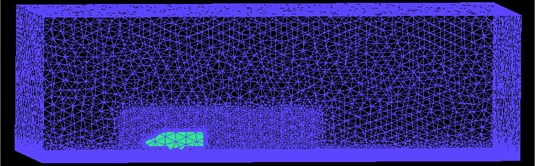
a) Aerodynamic meshes

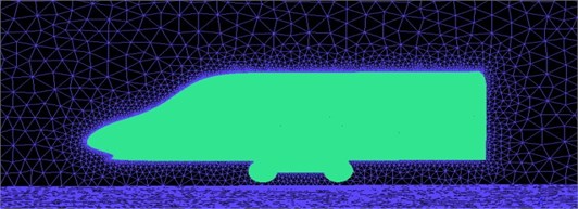
b) Local aerodynamic meshes

3.2. Results of aerodynamic characteristics for the high-speed transportation

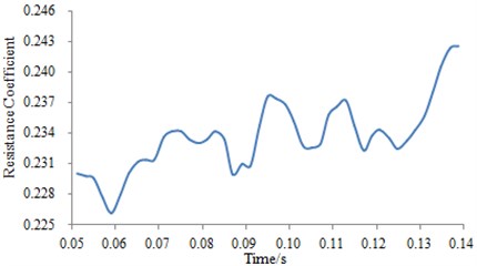
The resistance coefficient is defined as a dimensionless quantity, namely the ratio of the resistance and dynamic pressure of the airflow as well as the reference area. Its calculation formula can be found as follows:

7

C = \frac{X}{2 ρ υ^{2} S},

where $C$ is the resistance coefficient, and $X$ is the resistance, which is positive if the resistance has the same direction with the inflow, vice versa. $ρ$ is the air density, $υ$ is the velocity of the airflow relative to the object, and $S$ is the orthographic projection area of the object.

FLUENT software is applied in the paper to calculate the flow field of the high-speed transportation. In such process, the Monitor in the software can be adopted directly to solve the resistance coefficient. The changes of resistance coefficient are focused and expressed in the form of records and window. Finally, the resistance coefficient can be extracted directly from the software after completing the calculation, as shown in Fig. 2.

As can be seen from Fig. 2, a lot of peaks and valleys are appeared in aerodynamic resistance coefficient. In addition, an increasing trend is presented by the aerodynamic resistance coefficient with time goes by, which can be explained by the greater resistance effect caused by the increasingly contact area of some vortexes on the high-speed transportation. When the time is 0.125 s, the aerodynamic resistance coefficient is increased sharply because the airflow has gradually comprehensive acted on the high-speed transportation meanwhile. And the resistance coefficient will definitely reach a stable value when the time is increased to a certain extent.

Fig. 2Aerodynamic resistance coefficient on the surface of the high-speed transportation

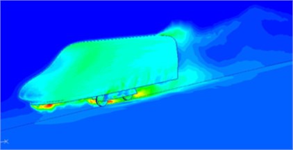
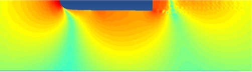
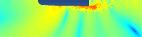
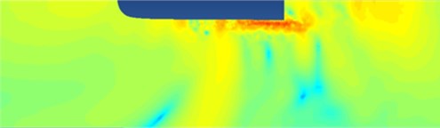
The pressure distribution on the high-speed transportation is shown in Fig. 3. Herein, greater pressure is presented on the bogie and nose tip of the head, namely the transition point of the geometric structure. Therefore, a certain separation vortex would be produced, resulting in airflow disorder on the high-speed transportation and thereby causing greater pressure.

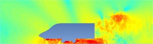
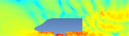
To further verify the above conclusions, the aerodynamic separation vortex is extracted from the high-speed transportation, whose result is shown in Fig. 4. As can be seen, more serious separation vortexes are appeared at the nose tip and bogies, indicating the reliability of the above analysis results.

Fig. 3Pressure distribution on the high-speed transportation

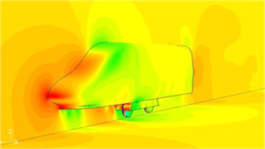
Fig. 4Separation vortex distribution on the high-speed train surface

4. Calculation of aerodynamic noise for the high-speed transportation

4.1. Aerodynamic noise of the high-speed transportation in the near field

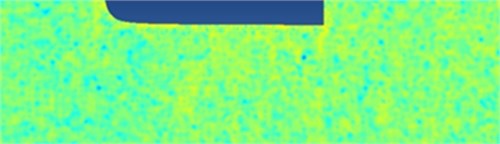
The aerodynamic characteristics result of the high-speed transportation obtained is then imported into ACTRAN software to establish the near acoustic field model as shown in Fig. 5. Furthermore, the turbulent sound source distribution of the high-speed transportation is calculated, with the result shown in Fig. 6. The frequency band within 1000 Hz is calculated in the figure, and only the medium and low frequency bands are analyzed. The distribution of high frequency components is almost completely missed due to the following reasons: 1) According to the theory of 1/6 Wavelength, the length of the element should be 50 mm at most if the upper limit of the frequency is 1000 Hz during the calculation of the sound field. Finally, 1463329 elements and 1595128 nodes are included in the entire model. As can be seen, numerous elements also need a very high requirement for the performance of the computer, which is hard to be satisfied by general computers. 2) As shown from the calculation results in Fig. 6, the noise source distribution is gradually weakened with the increasing frequency, and the intensity of the sound source has already been very small in the whole calculation area when the frequency reaches 1000 Hz. Therefore, the calculation results in the frequency band over 1000 Hz will be certainly smaller than that at 1000 Hz, whose researches thus have little significance. Therefore, only results within 1000 Hz are calculated in the paper in consideration of two factors.

Fig. 5Acoustic calculation model of the high-speed transportation

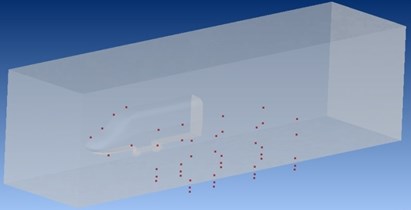
Fig. 6Turbulent sound source distribution on the high-speed transportation

a) 10 Hz

b) 50 Hz

c) 100 Hz

d) 1000 Hz

To further research the acoustic characteristics of the high-speed transportation under flow field, six observation points are arranged on the surface of the high-speed transportation, as shown in Fig. 7. In the figure, four observation points are in the longitudinal symmetrical plane of the high-speed transportation and the other two are placed on the lateral plane, which is easier for extracting sound pressure response of the high-speed transportation at different locations, thus convenient for analysis.

Fig. 7Distribution of observation points on the high-speed transportation

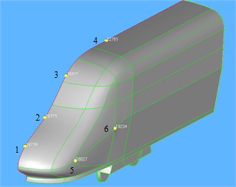
Fig. 8Sound pressure response of field points on the high-speed transportation

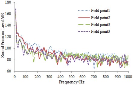
a) Longitudinal symmetrical plane of the high-speed transportation

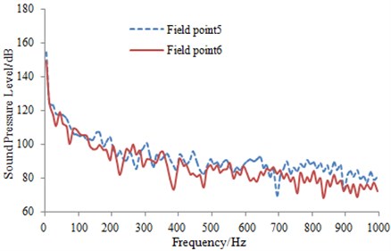
b) Lateral plane of the high-speed transportation

Based on the acoustic calculation model of the high-speed transportation, the sound pressure response at six field points is extracted with the results shown in Fig. 8. It is known that the pressure at field point 1 is largest as a whole mainly since its position is closest to the nose tip of the high-speed transportation.

According to the above analysis, the surface pressure is relatively large at this position, thus generating greater sound pressure response. In addition, the sound pressure response of the high-speed transportation is reduced gradually along with the increase of the calculated frequency, which further verifies the results in Fig. 6.

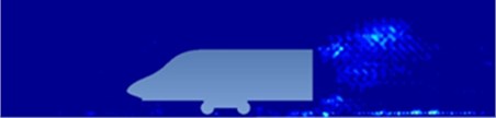
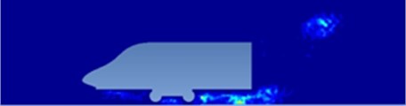
Fig. 9Sound pressure distribution on the high-speed transportation

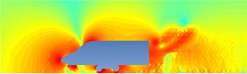
a) 10 Hz

b) 50 Hz

c) 100 Hz

d) 1000 Hz

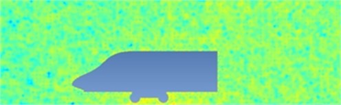
The sound pressure response contour on the high-speed transportation is extracted, whose results are shown in Fig. 9. As observed, the sound pressure decreases with the increasing frequency. In addition, the sound pressure is mainly distributed in the nose tip and bogies of the high-speed transportation, since the sudden change of these structures would cause vortex flow disorder, thereby generating larger noise.

4.2. Aerodynamic noise of the high-speed transportation in the far field

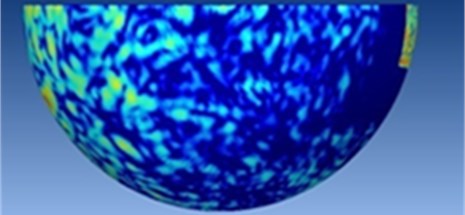
All of the above researches are related to aerodynamic noise on the high-speed transportation. However, researches are also necessary for the far-field sound pressure response. As shown in Fig. 10(a), an enveloped hemispheric mesh is built on the exterior side of the calculation model for the near field of the high-speed transportation.

Fig. 10Numerical computation of far acoustic field

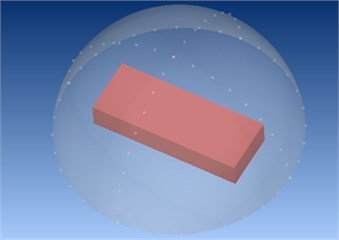
a) Simulation model

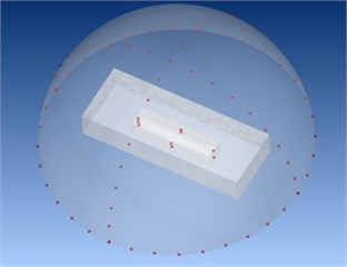
b) Field point

Fig. 11Far-field radiation noise of the high-speed transportation

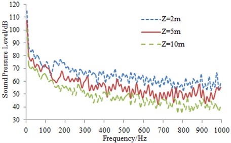
The sphere radius is 10 m in order to receive the far-field noise of the high-speed transportation. In a high-speed transportation, the propagation medium from the near-field to the hemispherical surface is air. In addition, many field points are set on the hemispherical mesh as shown in Fig. 10(b), in order to extract the curve of the radiation noise. SPL curves at the observation points of 2 m, 5 m and 10 m away from the longitudinally symmetrical plane of the high-speed transportation are extracted and thereby compared as shown in Fig. 11. The point of 2 m away from the longitudinally symmetrical plane is close to the high-speed transportation surface, with relatively large SPL. Along with the increasing larger distance between the observation point and the longitudinally symmetrical plane, SPL is decreased gradually. SPL has similar change trend at any position in the whole frequency domain, namely reducing gradually with the increasing frequency. The sound pressure contours are extracted at 50 Hz, 100 Hz and 1000 Hz, as shown in Fig. 12. It can be seen that the sound pressure is indeed reduced gradually with the increasing analyzed frequency, which is consistent with the above results.

Fig. 12Contours of far-field noise distribution for the high-speed transportation

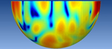
a) 50 Hz

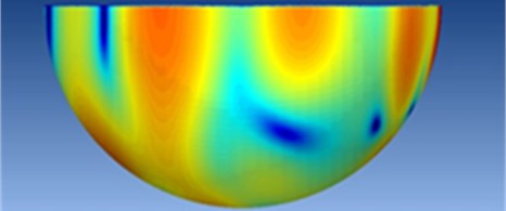
b) 100 Hz

c) 1000 Hz

5. Experimental verification of aerodynamic noise for the high-speed transportation

The high-speed transportation is a complicated model. Results of its aerodynamic noise may not be accurate if the research is conducted directly by a numerical method. Therefore, accuracy of the numerical calculation model shall be verified by experiment.

5.1. Experimental verification of aerodynamic noise in the near field

PULSE analyzer of B&K Company is used as test equipment in aerodynamic noise experiment of the high-speed transportation. During the test of the external sound pressure for a high-speed train under high-speed operation condition, a traditional microphone can’t be used to obtain the accurate experimental results. Therefore, a lot of aviation microphones are installed on the outer surface of the high-speed train to test the external sound pressure. To verify the numerical calculation result more accurately, the sensors are placed in positions of Fig. 7: four sensors are placed in the longitudinally symmetrical plane and two are set in the horizontal plane. In this way, the accurate experimental results can be obtained under high-speed operation. Test process of the external sound pressure is shown in Fig. 13. Multi-channel signal collection equipment is used to obtain signals of microphones. Then, the obtained data signals are imported into PULSE analyzer for the further processing. Sound pressure levels of high-speed train body surface under steady-state operation are finally obtained and compared with the corresponding simulation, as shown in Fig.14. It can be seen from the figure that the simulation is consistent with that of the experimental. The numerical calculation model is reliable and the above analysis is also accurate.

Fig. 13Test process of aerodynamic noise for the high-speed transportation

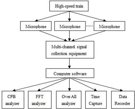
Fig. 14Comparison of aerodynamic noise between experiment and simulation

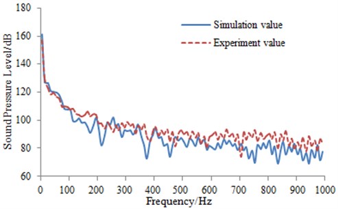
a) Longitudinal symmetrical plane of the high-speed transportation

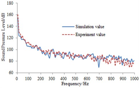
b) Lateral plane of the high-speed transportation

5.2. Experimental verification of aerodynamic noise in the far field

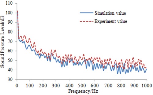
Far-field noise, also known as pass-by noise, has certain requirements for the selection of test site and arrangement of measuring points in order to ensure the test reliability of the pass-by noise. In-existence of large sound reflector is demanded in the three times of measuring distance surrounding the sensor. The acoustic absorption cover should be avoided as much as possible on the ground between the sensor and the measured high-speed transportation. There should be no rain or snow on the ground and the wind speed at 2 m above the track surface shall be no more than 8 m/s. The sensor needs to be placed perpendicular to the longitudinal symmetric plane of the high-speed transportation. The distance is not less than 5 m from the symmetric plane and the height is not less than 3 m away from the ground. As shown in Fig. 15, the placed sensor herein is 10 m away from the longitudinal symmetric plane and 7 m higher than the ground, satisfying the mentioned requirements. Finally, the experimental result is obtained and compared with that of the simulation, as shown in Fig. 16. It can be seen that the experimental values are substantially greater than the simulation value mainly because only aerodynamic noise is considered in the simulation calculation while the mechanical noise is not taken into account. However, the mechanical noise is included in the experimental result, and in addition, partial background noise is also existed in the experimental result. Resulted from two factors, the experimental result is generally greater than the simulation value. However, the proportion of mechanical and background noise is relatively small mainly due to the existence of aerodynamic noise under the high-speed operating condition. In addition, a relatively small effect of background noise is caused by the selection of testing environment and place. Therefore, experiment and simulation is of little differences in general, and the simulation model can still be used to predict far-field noise of the high-speed transportation.

Fig. 15Diagram of aerodynamic noise for the high-speed transportation

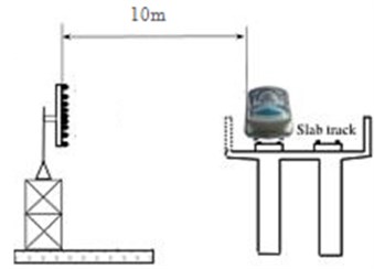
Fig. 16Comparison of aerodynamic noise between experiment and simulation

6. Conclusions

1) In the paper, DES method solved URANS equation in the near wall of the computational domain, and LES equation in the turbulent flow field away from the wall, whose mesh requirements and computation amount are between LES and URANS, which can better capture the unsteady sound source information that is necessary for the computation of aero-acoustics. Therefore, the advantage of small computation amount for URANS method can be performed in the boundary layer, and the large-scale separation vortices of LES method can be executed in the region away from the wall surface. Finally, not only the computational speed and efficiency are improved, but the computational accuracy is satisfied.

2) Aerodynamic characteristics of the high-speed transportation in the near field are calculated numerically. As shown from the corresponding result, due to the sudden structural changes of nose tip and bogies, their surface pressures are larger. Therefore, the numerical optimization of the aerodynamic characteristics for the high-speed transportation can be conducted from this aspect.

3) Based on the results of aerodynamic characteristics, the near-field and far-field aerodynamic noises of the high-speed transportation are also calculated. The near-field radiation noise is larger near the noise tip and bogies, while the far-field noise is greater near the ground.

4) The calculation results of the near-field and far-field for the high-speed transportation are verified by experiments, and they are consistent with each other. As a result, the numerical model established in the paper is reliable.

References

Shen Z. Y. Dynamic environment of high-speed train and its distinguished technology. Journal of the China Railway Society, Vol. 28, Issue 4, 2006, p. 1-5.

Search CrossRef
Talotte C. Aerodynamic noise: a critical survey. Journal of Sound and Vibration, Vol. 231, Issue 3, 2000, p. 549-562.

Publisher
Lighthill M. J. On sound generated aerodynamically: part 1: general theory. Proceedings of the Royal Society of London, Series A, Mathematical and Physical Sciences, Vol. 211, Issue 1107, 1952, p. 564-587.

Publisher
Curle N. The influence of solid boundaries upon aerodynamic sound. Proceedings of the Royal Society of London, Series A, Mathematical and Physical Sciences, Vol. 231, Issue 1187, 1955, p. 506-514.

Publisher
Ffowcs W. E., Hawkings D. L. Sound generation by turbulence and surfaces in arbitrary motion. Philosophical Transactions for the Royal Society of London, Series A, Mathematical and Physical Sciences, Vol. 264, Issue 1151, 1969, p. 321-342.

Publisher
Goldsten M. V. Unified approach to aerodynamic sound generation in the presence of boundaries. The Journal of Acoustical Society America, Vol. 56, Issue 27, 1974, p. 497-509.

Publisher
King W. F. A precis of development in the aeroacoustics of fast trains. Journal of Sound and Vibration, Vol. 193, Issue 1, 1996, p. 349-358.

Publisher
Noger C., Patrat Peube J. C. J. Aero-acoustical study of the TGV pantograph recess. Journal of Sound and Vibration, Vol. 231, Issue 3, 2000, p. 563-575.

Publisher
Li J. Q., He S. Q., Ming Z. An intelligent wireless sensor networks system with multiple servers communication. International Journal of Distributed Sensor Networks, Vol. 7, 2015, p. 1-9.

Publisher
Kitagawat T., Nagakurak K. Aerodynamic noise generated by Shinkansen cars. Journal of Sound and Vibration, Vol. 231, Issue 3, 2000, p. 913-924.

Publisher
Barsikow B. Experiences with various configurations of microphone arrays used to locate sound sources on railway trains operated by the DB AG. Journal of Sound and Vibration, Vol. 193, Issue 1, 1996, p. 283-293.

Publisher
Melleta C., Le’tourneauxa F., Poissonb F. High-speed train noise emission: latest investigation of the aerodynamic/rolling noise contribution. Journal of Sound and Vibration, Vol. 293, Issues 3-5, 2006, p. 535-546.

Publisher
Sassa T., Sato T., Yatsui S. Numerical analysis of aerodynamic noise radiation from a high-speed train surface. Journal of Sound and Vibration, Vol. 247, Issue 3, 2001, p. 407-416.

Publisher
Takehisa T., Akio S., Kiyoshi N. Numerical analysis of dipole sound source around high-speed trains. Railway Technical Research Institute, Vol. 111, Issue 6, 2002, p. 2601-2608.

Publisher
Takaishi T., Ikeda M. Method of evaluating dipole sound source in a finite computational domain. Railway Technical Research Institute, Vol. 116, Issue 3, 2004, p. 1427-1435.

Publisher
Xiao Kang Y. G. Z. C. Numerical prediction of aerodynamic noise radiated from high-speed train head surface. Journal of Center South University (Science and Technology), Vol. 39, Issue 6, 2008, p. 1267-1272.

Search CrossRef
Spalart P. R. Detached eddy simulation. Annual Review of Fluid Mechanics, Vol. 4, Issue 1, 2009, p. 181-202.

Publisher
Zhu Z. X., Xiao J., Li J. Q., Wang F. X., Zhang Q. F. Global path planning of wheeled robots using multi-objective memetic algorithms. Integrated Computer-Aided Engineering, Vol. 22, 2015, p. 387-404.

Publisher
Strelets M. Detached eddy simulation of massively separate flow. Proceedings of 39th AIAA Aerospace Science Meeting and Exhibit, 2001.

Publisher
Sreenivas K., Nichols D. S., Hyams D. G. Computational simulation of heavy trucks. Proceedings of 45th AIAA Aerospace Science Meeting and Exhibit, 2007.

Publisher
Mttchell A. M., Morton S. A., Forsythe J. R. Analysis of delta-wing vertical substructures using detached-eddy simulation. AIAA Journal, Vol. 44, Issue 6, 2006, p. 964-972.

Publisher

About this article

Received

08 September 2015

Accepted

06 April 2016

Published

15 May 2016

SUBJECTS

Acoustics, noise control and engineering applications

DOI

https://doi.org/10.21595/jve.2016.16397

Keywords

the high-speed transportation

aerodynamic characteristics

aerodynamic noise

Acknowledgements

This project is supported by Fundamental Research Funds for the Central Universities; Research Innovation Project of Shanghai Municipal Education Commission; Science and Technology Guidance Project of Chinese Textile Industry Association.

This is an open access article distributed under the Creative Commons Attribution License, which permits unrestricted use, distribution, and reproduction in any medium, provided the original work is properly cited.

Previous article in issue Previous Next article in issue Next

Research article

2017 09 30

Multi-objective optimization for the aerodynamic noise of the high-speed train in the near and far field based on the improved NSGA-II algorithm

Chun Yan Yuan, Ming Qing Li

Research article

2017 05 15

Numerical simulation of aerodynamic noises in the far field of the high-speed train with considering bogies and connection windshields

Wei-te Lu, Yan Wang, Chun-qin Zhang

Research article

2017 03 31

Research on the distribution of aerodynamic noises of high-speed trains

Wei Te Lu, Yan Wang, Chun Qin Zhang

Research article

2017 02 15

Numerical simulation and experimental study of aerodynamic noises for the cabin of the high-speed train

Ming Lv, Dong-er Xu, Hua He

Z. Tang, Z.- Liu, Q. Wang, and Z. Li, “Research on aerodynamic noise of the high-speed transportation based on experiment and simulation,” Journal of Vibroengineering, Vol. 18, No. 3, pp. 1954–1967, May 2016, https://doi.org/10.21595/jve.2016.16397

Copy Extrica

Copied to clipboard!

TY  - JOUR
DO  - 10.21595/jve.2016.16397
UR  - https://doi.org/10.21595/jve.2016.16397
TI  - Research on aerodynamic noise of the high-speed transportation based on experiment and simulation
T2  - Journal of Vibroengineering
AU  - Liu, Zhi-hui
AU  - Tang, Zhi
AU  - Wang, Qian
AU  - Li, Zhen
PY  - 2016
DA  - 2016/05/15
PB  - JVE International Ltd.
SP  - 1954-1967
IS  - 3
VL  - 18
SN  - 1392-8716
ER  - 

Copy Ris

Copied to clipboard!

@article{Liu_2016,
	doi = {10.21595/jve.2016.16397},
	url = {https://doi.org/10.21595/jve.2016.16397},
	year = 2016,
	month = {may},
	publisher = {{JVE} International Ltd.},
	volume = {18},
	number = {3},
	pages = {1954--1967},
	author = {Zhi-hui Liu and Zhi Tang and Qian Wang and Zhen Li},
	title = {Research on aerodynamic noise of the high-speed transportation based on experiment and simulation},
	journal = {Journal of Vibroengineering}
}

Copy Bibtex

Copied to clipboard!

[1]Z. Liu, Z. Tang, Q. Wang, and Z. Li, “Research on aerodynamic noise of the high-speed transportation based on experiment and simulation,” Journal of Vibroengineering, vol. 18, no. 3, pp. 1954–1967, May 2016, doi: 10.21595/jve.2016.16397.

Copy IEEE

Copied to clipboard!

Liu, Zhi-hui, Zhi Tang, Qian Wang, and Zhen Li. “Research on Aerodynamic Noise of the High-Speed Transportation Based on Experiment and Simulation.” Journal of Vibroengineering 18, no. 3 (May 15, 2016): 1954–67. https://doi.org/10.21595/jve.2016.16397.

Copy Chicago

Copied to clipboard!

Research on aerodynamic noise of the high-speed transportation based on experiment and simulation

Abstract

1. Introduction

2. Theory and computational boundary condition

3. Calculation of aerodynamic characteristics for the high-speed transportation

3.1. Aerodynamic mesh generation of high-speed trains

3.2. Results of aerodynamic characteristics for the high-speed transportation

4. Calculation of aerodynamic noise for the high-speed transportation

4.1. Aerodynamic noise of the high-speed transportation in the near field

4.2. Aerodynamic noise of the high-speed transportation in the far field

5. Experimental verification of aerodynamic noise for the high-speed transportation

5.1. Experimental verification of aerodynamic noise in the near field

5.2. Experimental verification of aerodynamic noise in the far field

6. Conclusions

References

About this article

Related Articles