Assessment of delaminations in composite beams using experimental frequencies

1. Introduction

Fibre-Reinforced Polymer (FRP) composites are widely used in aeronautical, marine and automotive industries, because of their excellent mechanical properties, low density and ease of manufacture. With increasing applications, it also becomes important to detect and study damage, which, in laminated structures, is mainly in the form of delaminations due to their low strength in the through-thickness direction [1].

There are many methods widely used for damage detection in engineering industries such as ultrasonic techniques, eddy-current technology and radiography. However, these traditional non-destructive inspection (NDI) methods are not applicable for Structural Health Monitoring (SHM) which requires the capability to monitor the integrity of the structure in real-time and in situ [2]. The SHM community has been putting continuous effort to develop strategies for detecting damage in operating structures. Vibration monitoring is one of the most promising ones since it uses dynamic parameters which can be easily and continuously extracted from the vibrations of a working machine [3]. The principle behind vibration based damage detection is that damage in a structure reduces the local stiffness which results in changes in dynamic parameters such as natural frequencies, mode shapes and damping ratios [4]. Therefore, by monitoring changes in these parameters we can detect and assess damage. The monitoring of mode shapes requires measurements at multiple locations, is time consuming and prone to noise. Damping parameters are notoriously difficult to measure, being sensitive to environmental conditions such as humidity and temperature. In comparison, natural frequencies require only single point measurement, and can be monitored with greater accuracy, ease and reliability [5]. However, while a shift in frequency easily identifies the presence of damage, the determination of the location as well as the severity of the damage is not easy to accomplish. It requires the solution of the inverse problem, viz., identifying the parameters indicating the location and severity of damage from measured changes in modal frequencies. Previous researchers have mainly resort to advanced system identification or optimization techniques such as neural networks [6, 7] and genetic algorithm [8]. Okafor et al. [7] used a theoretical model proposed by Tracy et al. [9] to generate a database relating frequency shifts to damage location and size in cantilever composite beams to train a neural network algorithm which is applied to predict delamination size from the measured frequency shifts in delaminated composite beams. Valoor and Chandrashekhara [10] trained a back propagation neural network to predict both delamination size and location by using the natural frequencies obtained from a thick beam model which incorporated shear deformation and Poisson effect.

However, when only two or three parameters are needed to assess the damage, such as location along the length of the beam, the depth at which it occurs and the size of a through width delamination, it can be easily determined using a graphical technique. The graphical technique was first proposed by Adams and Cawley [11], who showed that by plotting a crack size index versus crack location for the first three modes of a straight bar, the possible damage size and location can be estimated. Since then more researchers have employed a similar technique for solving the inverse problem, but mostly for estimating location and size of transverse or through thickness cracks in isotropic (metallic) beams [12-15] and there lacks a clear procedure description of how to apply this graphical detection method. In this paper, for the first time, the graphical approach is extended to detecting delaminations in orthotropic composite beams and a three-step process is developed for easy application. Besides, the existing theoretical model of delaminated beam [9] which is restricted to mid-plane delaminations has been extended to cover delaminations at other interfaces. Finally, the effectiveness of applying present method to assess the delamination in real beams has been validated by reported measured frequencies.

2. Methodology

The frequency shifts for each mode, between before and after delamination, is a function of both delamination size and location, which can be stated as a function:

where ‘$a$’ is delamination size, ‘$x$’ is delamination location along the beam length and ‘$n$’ is the mode number. The functions “$f_n$” are different for different modes and can be graphically depicted as three dimensional surface plots of “${\omega }_n$” as a function of “$a$” and “$x$” for each mode.

Assuming that we know natural frequency shifts due to a delamination in a laminated composite beam for several modes (either from measurement or numerical simulation), then a series of functions can be written as follows:

Since $\mathrm{\Delta }{\omega }_1$, $\mathrm{\Delta }{\omega }_2$, $\mathrm{\Delta }{\omega }_3$ are constants, we may rewrite the above functions as:

The curves represented by Eqs. (5)-(7) on the size-location plane will have a common intersection point since the frequency shifts ${∆\omega }_1$, $∆{\omega }_2$, ${∆\omega }_3$,…, have all been caused by the same delamination with specific values for its location and size.

The above procedure can be summarized into three steps as follows:

Step 1: Create surface plots of frequency shifts as functions of delamination size “$a$” and location along the beam length “$x$” for each mode (data can be obtained from theory, FE or experimental testing).

Step 2: Draw planes representing constant values of the known frequency shifts (can be from theory, FE or measurements) in each mode and find their intersections with the corresponding surface plots.

Step 3: Replot the intersection curves of all modes on the size vs. location plane, and find the point at which all curves intersect.

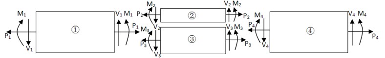
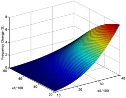
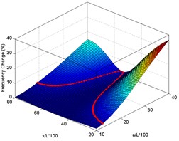
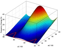
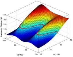
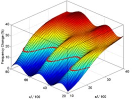
Steps 1 to 3 are illustrated with a typical example in Figs. 1 and 2. The surface plots of the frequency shifts as functions of the normalized delamination size over the beam length “$a/L$” and normalized location “$x/L$” for an eight-layer [0/90/90/0]_s Carbon fibre reinforced plastic (CFRP) cantilever beam are shown in Fig. 1 for modes 1, 2 and 3, respectively (Step 1). The database required for plotting the 3-D figures is obtained from theoretical model of delaminated beam (refer to next session). Also shown in the figures are curves indicating the intersection of each surface plot with the planes representing constant “measured” values of frequency shift in the corresponding modes (Step 2). The ‘measured’ frequency shift is obtained from the theoretical model as well. The intersection curves are replotted together in the size-location domain with “$x/L$” along the $x$-axis and “$a/L$” along the $y$-axis (Step 3) in Fig. 2. As can be seen all these curves intersect at one point which indicates the location and size of the delamination.

Fig. 1Surface plots of frequency changes with damage size and location for mid-plane delamination for first three modes and intersection of planes with known frequency shifts (Steps 1 and 2)

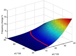
a) Mode 1

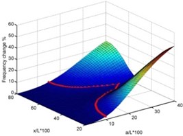
b) Mode 2

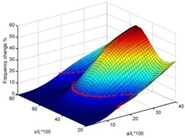
c) Mode 3

Fig. 2Intersection curves of modes 1 to 4 for determination of delamination size and location (Step 3)

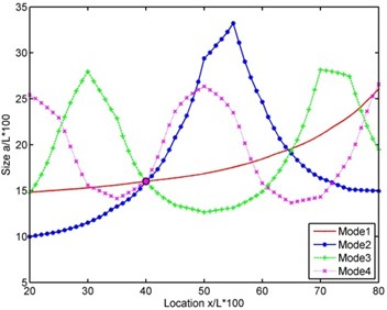
In a real situation, all the curves may not pass through a single point but form a small area due to measurement errors or discrepancy between the theoretical/FE models and the real beam. Thus, it is more expedient to replace the intersection point with the point at which the curves come closest to one another, and this is realized by calculating the minimum standard deviation of the distance from point to the curves.

3. Theoretical model

The earliest model for vibration analysis of composite beams with delaminations was proposed by Ramkumar et al. [16]. They modelled a beam with one through-width delamination by modelling four Timoshenko beams: two for the undelaminated segments and one for each sublaminates in the delaminated segment. Natural frequencies and mode shapes were determined by solving a boundary eigenvalue problem, after ensuring boundary conditions and continuity conditions at the edges of the delamination. Their predicted natural frequencies were consistently lower than the experimental results. Ramkumar et al. suggested that the inclusion of contact effect may improve the analytical prediction since they assumed the sublaminates vibrate freely. Instead of taking this suggestion, Wang et al. [17] improved the analytical solution to be closer to test results by including the coupling between flexural and axial vibrations of the delaminated sub-laminates. Subsequently, Mujumdar and Suryanarayan [18] imposed a constraint between the delaminated parts to have the same flexural deformations which is referred as the “constrained model” and validated their model with experimental results on isotropic beams. Tracy and Pardoen [9] has reported a similar constrained model to obtain the natural frequencies for a simply-supported composite beam. However, their model is restricted to mid-plane delamination only. In the present work, we have modified Tracy and Pardoen’s model to make it applicable to laminated composite beams with delaminations at any interface.

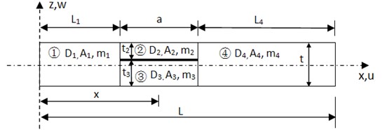
The simplified engineering beam model in which the delaminated beam is divided into four segments is shown in Fig. 3. Each segment is characterized by extensional stiffness $A_i$, bending stiffness $D_i$, and mass density per unit length $m_i$ ($i=$ 1-4). The model represents a delaminated beam of unit width, thickness $t$, and total length $L$. The delamination is located at distance $t_2$ from the upper surface of beam and the lengthwise location of the mid-point of the delamination is at “$x$” from the left end while the delamination size is “$a$”.

Fig. 3Delaminated beam model

The governing differential equation for each segment is [9]:

where $w_i$ is flexural displacement of $i$th beam segment, and $\omega$ is the natural frequency. By inspection of Fig. 3, note that the axial forces $P_1=P_4=$0, so that $P_2=-P_3$. The displacement functions $w_i$ which is solution to Eq. (8) have the form:

where:

It is helpful to reformulate the problem in terms of dimensionless parameters as follows [9]:

Now, Eq. (9) can be written as:

where $a_i^4={\overline{m}}_i/{\overline{D}}_i$, ${\overline{k}}^4=m{L}^4{\omega }^2/D$. In the constrained model proposed by Tracy and Pardoen [9], the mass to stiffness ratios of the segments 2 and 3 are set to be equal ($a_2=a_3$), so as to make their deflections $w_2$ and $w_3$, the same. However, this restricts their theoretical model applicable to beams with mid-plane delaminations only. In the present work, such restriction does not exist anymore since the two delaminated segments are directly constrained to have the same transverse displacement ($w_2=w_3$), instead of constraining the two sub-laminates of damaged part to have the same mass, thickness or stiffness. Therefore, it is reasonable to replace $w_2$ and $w_3$ in Eq. (11) with $w_d$ and this gives:

where $a_d^4={\overline{m}}_d/{\overline{D}}_d$, ${\overline{m}}_d=m_2+m_3/m$, and ${\overline{D}}_d=D_2+D_3/D$.

With this replacement, there are three flexural deflection $w_i$ ($i=1,\mathrm{}d,\mathrm{}4$), each with four coefficients $C_{i1}$ to $C_{i4}$. Hence, a total of 12 boundary and continuity conditions are required to construct 16 equations for the solution of all the unknown coefficients.

For a cantilever beam, the clamped-free boundary conditions at its ends are employed, that is, at $s=$ 0: $w_1=\mathrm{}0$, $d{w}_1/Lds=0$ and at $s=$ 1: $d^2{w}_4/L^{2}d{s}^2=0$, $d^3{w}_4/L^{3}d{s}^3=0$.

The continuity conditions between the undamaged and delaminated beam segments are, at $s_1=x_1/L$: $w_1=w_d$, $d{w}_1/Lds=d{w}_d/Lds$, $V_1=\mathrm{}{V}_2+\mathrm{}{V}_3$ and $M_1=\mathrm{}{M}_2+\mathrm{}{M}_3+\mathrm{}{P}_d\left(t/2\right)$, and at $s_2=x_2/L$: $w_4=w_d$, $d{w}_4/Lds=d{w}_d/Lds$, $V_4=\mathrm{}{V}_2+\mathrm{}{V}_3$ and $M_4=\mathrm{}{M}_2+\mathrm{}{M}_3+\mathrm{}{P}_d\left(t/2\right)$ while $P_d$ indicates the absolute values of the axial forces in the beam segments 2 and 3. the bending moment $M_i$ and the shear force $V_i$, are, respectively [9]:

According to [18], under the assumption that $w_2=w_3=w_d$, the axial force, $P_d$, can be obtained from the axial strains which can be determined in terms of the gradients of the transverse deflections at the connecting points, $s_1$ and $s_2$, as:

Substituting the displacement functions, $w_i$, from Eq. (11) and axial force, $P_d$, from Eq. (13) into the 12 boundary and continuity conditions of a cantilever beam, a set of 12 simultaneous linear homogeneous algebraic equations for the 12 unknown constants can be expressed in matrix form as:

where ${\mathbf{Q}}_{ij}\left(\overline{k}\right)$ are the coefficients of the unknown constants and ${\mathbf{V}}_j$ the column vector containing the 12 unknowns following the order of $C_{i1}$ to $C_{i4}$ for $i=$ 1, d, 4. For a non-trivial solution, the determinant of the coefficient matrix ${\mathbf{Q}}_{ij}\left(\overline{k}\right)$ must equal zero. The function ‘fzero’ in Matlab is used to determine the $\overline{k}$ values which make the matrix determinant zero. Then, the modal frequencies of the delaminated beam can be calculated from $\overline{k}$ since ${\overline{k}}^4=m{L}^4{\omega }^2/D$. Once the ${\mathbf{Q}}_{ij}$ coefficients are known, the elements of the displacement vector, ${\mathbf{V}}_j$, can be calculated to obtain the displacement function for each beam segment which provide the theoretical mode shapes of the delaminated beam.

4. Experimental validation

Experimental data of frequency measurements on delaminated beams is very hard to come by in literature, possibly due to the difficulty of manufacturing laminated composite beams with simulated delaminations. Of the three published test results that the author could find, only one sample in one publication had off-mid-plane delamination [19]; all the others have simulated delaminations in the mid-plane. The validity of the proposed graphical method for damage detection is verified using experimental data from these three publications: Grouve et al. [20], Okafor et al. [7] and Su et al. [19]. The results are presented in the following sub-sections.

4.1. Experimental validation using measured frequencies reported by Grouve et al. [20]

Experimental results from published literature are employed to validate the proposed graphical detection method. Grouve et al. [20] conducted modal testing of 16-ply ([90/0/90/02/90/0/90]_s) cantilever glass/epoxy beams with and without mid-plane delaminations. A total of five beam specimens were manufactured, with one perfect sample (A1) and four delaminated samples (A2, A3, A4 and A5) in which the delaminations were created by placing a thin (<16 μm) foil of polyimide between two plies prior to curing process. The delaminations were all embedded at mid-plane of the four delaminated specimens, with the normalized length-wise location and size ([$x/L$, $a/L$]) being [52 %, 20 %], [52 %, 30 %], [32 %, 20 %], [32 %, 30 %] for specimens A2 to A5, respectively. Basically, Grouve et al. have studied delaminations of two locations along the beam (namely 52 % and 32 % of whole beam length from the fixed end) and of two sizes (30 % and 20 % of whole beam length), but only of one interface, i.e. the mid-plane, in their experimental work.

The percentage shift in frequency in the $i$th mode were calculated by:

$∆{\omega }_i=\frac{{\omega }_{ui}-{\omega }_{di}}{{\omega }_{ui}}\times 100,$

where ${\omega }_{ui}$ and ${\omega }_{di}$ are the $i$th mode frequency of the undelaminated and delaminated beams, respectively. The frequency shifts for each delaminated beam sample calculated from the measured values in [20] are then presented in Table 1.

Table 1Experimental frequency changes of composite beams in [20]

Mode No.	Measured frequency change (%)
	Case 1 (A2*)	Case 2 (A3)	Case 3 (A4)	Case 4 (A5)
Mode 1	–9.09	–9.09	–9.09	–9.09
Mode 2	–5.26	–9.21	2.63	14.47
Mode 3	9.95	23.08	0.45	5.88
Mode 4	–1.85	3.47	14.12	21.53
Mode 5	18.99	23.74	14.94	25.14
Mode 6	7.02	23.88	8.33	27.43
*A2~A5 are the specimen ID in [20]

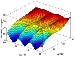
As the first step, the functions of frequency shift with normalized delamination size $a/L$ (10 %-40 %) and location $x/L$ (20 %-80 %) are plotted as 3D surfaces (Fig. 4). The curve appearing in each of these surface plots is the intersection of the plane representing the measured value of frequency shift of case 3 beam with the surface plot for that mode.

Fig. 4Surface plots of frequency changes with delamination size and location for experimental delaminated beam for first six modes (using case 3 measured data for drawing intersection curves)

a) Mode 1

b) Mode 2

c) Mode 3

d) Mode 4

e) Mode 5

f) Mode 6

Fig. 5Intersection curves plotted together for determination of intersection point for four experimental test cases in [20]

a) Case 1

b) Case 2

c) Case 3

c) Case 4

Fig. 5 shows the results of the final step of graphical detection where all the intersection curves are plotted together to get the intersection point. As mentioned before, the intersection curves may not perfectly pass through a single point due to measurement errors or mismatch between the theoretical model and real beam. Therefore, the intersection point is determined by calculating the point which gives the minimum standard deviation of distance between point and the curves, viz., where the curves come closest to one another. The coordinates of those points in Fig. 5 indicate the predicted delamination size and location. The comparison between the predicted and the actual delaminations size and location is shown schematically in Fig. 6, with the actual [20] and predicted delaminations represented by green and yellow rectangles drawn to scale, on the left and right side beams, respectively. As can be seen, good prediction of both delamination size and location is achieved; especially for the location prediction, the prediction errors are below 4 %. The errors may stem from the discrepancy between the theoretical model and the real beam due to manufacturing imperfections, e.g., the final size of artificial delamination in the composite specimens may be smaller than the designed length since the laminates are not separated thoroughly around the damage edge; or there may be small inaccuracies in the ply orientations. There is also the possibility that the presence of the release film may slightly alter the stiffness of the composite laminate. In addition, there is uncertainty and errors involved in the measurement of frequencies. Taking into account all these factors, we can conclude that the accuracy of the proposed graphical detection method is very good and that it can be applied to detect and assess delamination size and location successfully in laminated composite beams.

Fig. 6Actual (left) and predicted (right) delamination for tested cases in [20]

a) Case 1

b) Case 2

c) Case 3

d) Case 4

4.2. Experimental validation using measured frequencies reported by Okafor et al. [7]

Okafor et al [7] manufactured and tested four eight-layer ([0/90/90/0]_s) glass/epoxy cantilever beams, one control sample and the other three with mid-plane delaminations. The distance between the center of the delamination and the clamped end is 11.75 cm for all three delaminated beam specimens (full length is 26.67 cm). Delamination has covered a length of 5.08 cm, 10.16 cm, and 15.24 cm of the three damaged beams respectively. Thus, the normalized delamination parameters ([$x/L$, $a/L$]) of the three damaged beam samples reported by Okafor et al. are [44 %, 19 %], [44 %, 38 %], [44 %, 57 %]. The changes in the measured frequencies of the three delaminated specimens from those of the undelaminated beam are given in Table 2 for the first four modes.

As can be seen, the frequency changes in the first two modes in cases 1 and 2 are negative suggesting that the frequencies of delaminated beam are higher than those of the undamaged one which is not theoretically possible and can possibly be attributed to errors in measurement or differences in beam properties between the delaminated and undelaminated samples. These measurement errors make the data not sufficient to obtain only one intersection point by present graphical detection method for case 2 (as can be seen in Fig. 7).

Table 2Experimental frequency changes of composite beams in [7]

Mode no.	Measured frequency change (%)
	Case 1 (5.08 cm*)	Case 2 (10.16 cm)	Case 3 (15.24 cm)
Mode 1	–6.67	–6.67	6.67
Mode 2	–6.19	–1.03	15.46
Mode 3	5.49	18.32	32.97
Mode 4	2.24	17.57	31.03
* delamination length

Fig. 7Intersection curves plotted together for determination of intersection point for three experimental test cases in [7]

a) Case 1

b) Case 2

c) Case 3

However, we are still able to make a reasonable prediction by present insufficient data. the comparison of the prediction accuracy between by graphical detection method and by the neural network reported in [7] is displayed in Tables 3-5. As can be seen, the predicted errors are smaller compared to the prediction reported by Okafor et al.

Table 3Delamination size prediction in composite beam with 5.08 cm delamination

Case 1	Predicted size (cm)	Error (%)
Present prediction	4.89	–3.82 %
Prediction in [7]	5.33	0,05

Table 4Delamination size prediction in composite beam with 10.16 cm delamination

Case 2		Predicted size (cm)	Error (%)
Present prediction	Left point	9.76	–1.52 %
	Right point	9.13	–3.76 %
Prediction in [7]		10.57	0,04

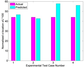
Beside the size, the location of the delamination can also be predicted at the same time using present graphical method, while the neural network trained by Okafor et al. only determined the delamination size. the comparison between the actual and predicted locations is illustrated schematically in Fig. 8. Since there are two intersection points in case 2, both predictions are plotted: 2 for left point and 3 for the right one. Considering the insufficient data available for the graphical method, the location prediction is reasonably good.

Table 5Delamination size prediction in composite beam with 15.24 cm delamination

Case 3	Predicted size (cm)	Error (%)
Present prediction	15.08	–1.06 %
Prediction in [7]	18.14	19 %

Fig. 8Comparison between actual and predicted location of delamination (2 and 3 in x axial indicate the prediction from two intersection points in case 2)

4.3. Experimental validation using measured frequencies reported by Su et al. [19]

Su et al. [19] conducted modal testing on five 10-layer ([0/90/0/90/0]_s) woven glass fibre reinforced composite beams, with one intact beam (specimen ID in [19]: SP0) as benchmark, three beams with mid-plane delaminations (SP1, SP3, SP4), and one beam with an off-mid-plane delamination (SP2), i.e. locating at the second interface from the outer surface. the delamination locations $x/L$ and sizes $a/L$ are [17.5 %, 25 %], [50 %, 25 %], [50 %, 25 %], [50 %, 40 %] for SP1-SP4, respectively. the first three measured frequencies are given in [21] and the calculated frequency changes are listed in Table 6.

The three steps of the graphical method, viz., creating surface plots, finding the curves of their intersections with the planes representing measured frequency shifts, and replotting the intersection curves for different modes to find the point of maximum proximity (minimum standard deviation) between them. It is to be noted that for the beam with the off-mid-plane delamination (Case 2), the frequency data for the surface plots in step 1 was obtained from the modified theoretical model applicable off-mid-plane delaminations described in Section 3.

Table 6Experimental frequency changes of composite beams in [19]

Mode No.	Measured frequency change (%)
	Case 1 (SP1*)	Case 2 (SP2)	Case 3 (SP3)	Case 4 (SP4)
Mode 1	6.29	0.22	0.90	1.57
Mode 2	7.48	3.07	17.76	12.02
Mode 3	4.54	0.19	12.04	9.91
*SP1~SP4 are specimen IDs in [19]

Fig. 9 shows the results of step 3 for cases 3 and 4. as can be seen, the intersection curves are symmetrical due to the clamped-clamped boundary condition; and therefore there are two possible locations for the damage, one on either side of the mid-section of the beam. This is not a drawback of the inverse algorithm, but a limitation of the fact that we are using frequency data from a beam with symmetrical boundary conditions because a damage located at the same distance on either half of the beam will create the same shift in frequency since all the modes are either symmetric or antisymmetric for a beam with symmetric boundary conditions.

Fig. 9Intersection curves plotted together for determination of intersection point for experimental cases in [19]

a) Case 3

b) Case 4

Fig. 10Actual (left) and predicted (right) delamination for tested cases in [19]

a) Case 1

b) Case 2

c) Case 3

d) Case 4

The comparison between the actual and predicted locations for this case study is illustrated schematically in Fig. 10 as can be seen, the predictions are not as good as those obtained in the first case study, with experimental data from Grouve et al. [20]. The larger discrepancy in the present case is possibly due to having only the first three measured modal frequencies. It is also should be noted that the fundamental frequency is usually very difficult to measure accurately; and hence lead to greater inaccuracies if used for damage assessment. in general, it is better to use as many higher modes as possible in the inverse algorithm for detection to improve accuracy.

5. Conclusions

A simple three-step graphical detection method using frequency measurements is developed for detecting and assessing delaminations in composite beams. the validation using three different sets of experimental data shows that this method can be successfully employed to predict the delamination size and lengthwise location in real composite beams with good accuracy. in the theoretical model for delaminated beam, a previous theoretical model has been extended to make it applicable to beams with delaminations at any interfaces. Since the proposed graphical method only requires measured shifts in natural frequencies, it has the potential to detect delamination propagation through continuous monitoring. Therefore, present graphical method has promise for future applications in Structure Health Monitoring of composite structures.