Aerodynamic characteristics of multiple flapping wing configurations

Shen, Yuan; Cai, Hongming

doi:10.21595/jve.2016.16568

Journal of Vibroengineering

Browse Journal

Submit article

Published: 15 May 2016

Check for updates

Aerodynamic characteristics of multiple flapping wing configurations

Yuan Shen¹

Hongming Cai²

¹Nanjing University of Aeronautics and Astronautics, Nanjing, P. R. China

²Nanjing University of Science and Technology, Nanjing, P. R. China

Corresponding Author:

Hongming Cai

Cite the article Download PDF

Downloads 1952

WoS Core Citations 6

CrossRef Citations 6

Abstract

Natural flyers and man-made MAVs generally use multiple flapping wing configurations. To understand the aerodynamic performance, three different flapping configurations: single wing, tandem wings, and biplane wings are numerically simulated by a URANS solver coupled with an overset grid method. Moreover, effect of kinematics including oscillating frequency, angle of attack and wing to tail distance are detailed investigated. Results show that the wing-tail interaction significantly benefits the thrust generation when the wings are tandem arranged. Additionally, the tandem arrangement is the most efficiency configuration when applied with high frequencies. Biplane wings model has the most inefficiency propulsive performance, nevertheless it can provide an extensive aerodynamic force. With the increasing AOA, biplane has the largest critical angle from thrust to drag. Wing-tail interaction becomes weaker when the tail is mounted further from the flapping wings. The present of the tail in tandem model bring more benefits compared with the tail in biplane model. The tail in biplane model is only functional for flight control when applied with a non-zero angle of attack.

1. Introduction

Of all locomotion, nature created flying is always the most fascinating one due to its outstanding flight efficiency and maneuverability. Birds, insects and cetaceans use their flapping wings or body system to solely generate both lift and thrust. Recently, the development of micro air vehicles (MAVs) has stimulated the interest in flapping motion. There is therefore an increased desire to provide a deeper insight into the aerodynamic mechanisms of flapping flight and how they may be adopted or integrated for the design of flapping MAVs. Ultimately, it is always essential to offer the designers and engineers a clear picture about the overall aero/hydrodynamic knowledge and useful tools to organize the flapping mechanism which is most suitable for specific mission objective and flight envelop.

Studies about the flapping mechanisms have been extensively reported in the literature. The thrust generated by an oscillating wing was first observed by Knoller [1] in 1909 and similar work has been done by Betz [2] in 1912. They observed that a wing performing a sinusoidal oscillating motion in a free stream can generate both lift and thrust, which is now known as the Knoller-Betz effect. The Knoller-Betz effect was firstly verified experimentally by Katzmayr [3] in wind tunnel tests at the Technical University of Vienna. Garrick [4] published a set of equations for thrust and efficiency of the flapping wing based on flat-plate theory. Von Karman and Burgers [5] firstly gave the theoretical explanation for the drag and thrust of the flapping wings, by relating it to the observed shape and orientation of a double row of counter rotating vortex pairs in the wake, i.e., the von Karman vortex street. Based on thin airfoil theory, Garrick [4] indicated that the propulsive efficiency of purely plunging airfoils drops rapidly from values close to one at low frequencies to close to 0.5 as the frequency is increased. Nevertheless, the foregoing research has been largely limited to configurations of a single airfoil that could flap in pure plunge, pure pitch and a combination of plunge-pitch mode. In view of this, the prediction of single oscillating airfoil or wing behavior becomes relatively simple, based on the accumulated data base. However, due to the limitations in manufacturing precision, materials and miniaturization, artificial ornithopters cannot fly as good as natural flappers. That is the reason that only few of the existing flapping MAVs adopt the single wings mode which the natural flyers use. In contrast, tandem and biplane configurations are widely used in flapping MAVs, such as “DelFly” [6, 7], to obtain extra aerodynamic forces, high propulsive efficiency and reliable control capability. Understanding and predicting of the aerodynamic characteristics interaction between wing and tail or between the close coupled wings therefore becomes essential.

The present study addresses a numerical study on the aerodynamic characteristics of multiple flapping wing configurations, by using an overset grid technique proposed by Deng et al. [8] to guarantee mesh quality when large deformation happens. Three different two-dimensional flapping configurations are considered: 1) single wing with a combined plunge-pitch mode, 2) tandem arrangement with a stationary tail and 3) biplane configurations with two opposed flapping wings as well as a tail. In this investigation a parametric study is performed to reveal the effect of the reduced frequency, angle of attack and wing to tail distance. All wing and tail elements are represented by a NACA0012 airfoil. The oscillation motion is prescribed with a combination of plunging and pitching. Aerodynamic characteristics includes the propulsive performance, lift enhancement and wing to tail interaction are numerically predicted and analyzed. This paper is organized as follows. In Section 2 the methodologies employed in this paper are presented and further verified and validated in Section 3. Subsequently, the computational set up for the three different flapping models are described in Section 4. Numerical results of the aerodynamic characteristics are performed in Section 5, followed by conclusions in Section 6.

2. Numerical methodology

2.1. Arbitrary Lagrangian Eulerian Navier-Stroke equations

For the general problem of compressible flows in a moving and deforming computational domain $Ω$ , the integral form of unsteady compressible Navier-Stroke equations can be written as:

1

Γ_{W} \frac{\partial}{\partial τ} \int_{Ω (t)}^{} W d V + \frac{\partial}{\partial t} \int_{Ω (t)}^{} W d V + \oint_{S (t)}^{} F (W - v_{g} W) d S = \oint_{S (t)}^{} F_{v} d S,

where $W = {(ρ, ρ u, ρ v, ρ w, ρ e)}^{T}$ , $F (W)$ and $F (v)$ represent the convective and viscous fluxes. $Γ_{w}$ is the low Mach preconditioning matrix [9], which allows obtaining efficient and accurate solutions at low Mach numbers. In order to obtain meaningful solutions for unsteady flow, it is necessary to use a pseudo time approach. It is therefore $τ$ and $t$ in Eq. (1) are the pseudo and physical times. Defining $v_{g} = \dot{x} ∙ \vec{n}$ , where $\dot{x} = (u, v, w)$ corresponds to a Lagrangian system, and $v_{g} =$ 0 is a Eulerian one. In the present formulation, $v_{g} =$ 0 is arbitrarily specified.

The in-house solver used in the present study can be operated on any type of mesh, viz. structured, unstructured and Cartesian or hybrid of them. The solver is spatially discretized by a unified method for cell-centered and vertex-centered scheme. The inviscid flux through the interface between the adjacent control volumes is calculated using a reformulated Roe-type flux difference splitting scheme. The pseudo time term $τ$ in Eq. (1) is temporally discretized with a first order backward difference and the physical time term $t$ is discretized in an implicit fashion by means of 2-step backward difference respectively. A detail description of the in-house programmed CFD solver can be found in [10]. The Reynolds numbers in the present computations are all set at 10,000, hence the laminar flow is considered.

2.2. Aerodynamic force and power calculation

The time-averaged aerodynamic force and power in the present research are defined as:

2

\bar{F} = \frac{1}{T} \int_{0}^{T} \int_{S}^{} F (t) d A d t, \bar{P, a} = \frac{1}{T} \int_{0}^{T} \int_{S}^{} F (t) \dot{x} d A d t,

where $F (t)$ is the aerodynamic force of a wall element. Furthermore, the thrust coefficient $C_{T}$ , aerodynamic power coefficient $C_{P, a}$ , and the propulsive efficiency (the ratio of thrust coefficient to power coefficient) $η$ are given respectively by:

3

C_{T} = \frac{- F_{x}}{0.5 ρ U_{\infty}^{2} c}, C_{P} = \frac{- F_{x}}{0.5 ρ U_{\infty}^{3} c}, η = \frac{\bar{C_{T}}}{\bar{C_{p, a}}},

where $U_{\infty}$ and $c$ are the incoming free-stream velocity and the chord length.

3. Solver verification and validation

An airfoil that oscillates in plunge motion is considered in this section to assess the verification and validation of the solver as well as the overset grid technique we developed. Experimental and numerical results from literatures are employed for computational validation.

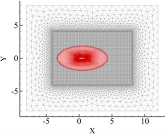
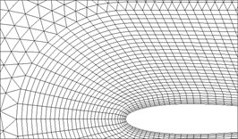
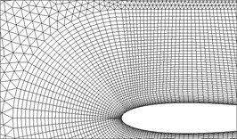
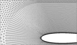
In order to test the grid and time step sensitivity, the unsteady flow of a purely plunging NACA0014 airfoil is computed under conditions of $k =$ 2, $H_{0} =$ 0.4 $c$ , and $R e =$ 10,000. During the test, three mesh models with different resolutions (seen in Fig. 1(b)-(d) and Table 1) are considered over a same background Cartesian mesh (Fig. 1(a)). Moreover, three different inner time steps (20, 50, 100) are also evaluated.

Fig. 1a) The overset grid setup of the plunging NACA0014 airfoil and the near views of the three different resolution in Table 1 (Mesh A to C)

a)

b)

c)

d)

Table 1Grid refinement case

Mesh model	Resolution	Grid size	1st BL height
Mesh A	40×30	9597	0.0005c
Mesh B	80×40	26292	0.0002c
Mesh C	160×60	59409	0.0001c

Fig. 2 shows the drag coefficients history of the mesh and time step refinement versus with non-dimensional time, respectively. For a further validation, computation results from Tuncer & Kaya [11], and Miao & Ho [12] are also plotted in Fig. 2 (a). It is evident that the present solver can spatially and temporally guarantee the numerical accuracy.

Fig. 2Drag coefficients history vs. non-dimensional time

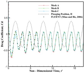
a) Mesh refinement

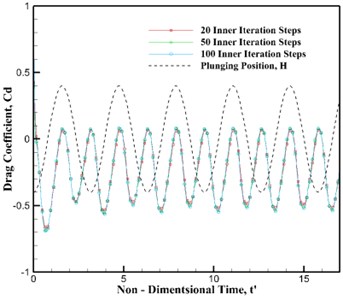
b) Time step refinement

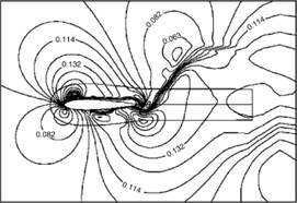
Fig. 3(a) presents the computed Mach contour when the airfoil plunged at the middle position, while Fig. 3(b) and (c) are the results from Ref. [11, 12]. Obviously, all the Mach contours reach a good agreement, which confirms that the code is capable of capturing the flow details at the desired level of accuracy.

Fig. 3Mach number contour at t=3/4T (middle position)

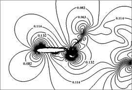
a) Computed by overset grid in present study

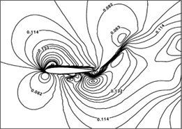
b) Computed by conformal hybrid-grids, adapted from Ref. [8]

c) Computed by overset grid, adapted from Ref. [7]

4. Flapping wing kinematics and computational set-up

In present study, three different flapping models are considered: (a) Single airfoil in an oscillating model; (b) Tandem model with an oscillating forward wing and a non-oscillating rearward wing; (c) Biplane model with two opposed oscillating wing and a stationary tail which is corresponded to the configuration of the DelFly onithopter. The flapping kinematics used in this study is a combination of sinusoidal pitching and sinusoidal plunging, with pivot point at quarter-chord location from the leading edge. Fig. 4 illustrates the three flapping models, the plunge and pitch motion equations are given by Eqs. (4) (5), respectively:

4

H (t) = H_{0} \sin (2 π f t),

5

α (t) = α_{0} \sin (2 π f t + ϕ),

where $H_{0}$ and $α_{0}$ are the plunging and pitching amplitudes, respectively, while $ϕ$ stands for the phase lag between pitch and plunge motion. Anderson et al. [13] pointed that the propulsive efficiency reached a maximum at $ϕ =$ 90°, hence, the phase lag $ϕ$ of all the computations in present study is set at 90°.

For each flapping wing, the plunging amplitude is 0.4 $c$ , pitching amplitude is 5°, wing to tail distance stays at 0.5 $c$ and for biplane configuration the mean wing to wing distance is 1.2 $c$ in order to prevent the airfoils crossing each other.

Fig. 4Three different flapping models

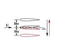
a) Single wing

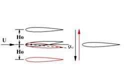
b) Tandem wing

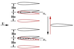
c) Biplane wing

5. Results and discussions

5.1. Effect of wing to tail interaction

Taylor [14] reported that the propulsive efficiency for the flying and swimming animals peaks at about Strouhal Number $(S t) =$ 0.29. It is therefore $S t =$ 0.29, corresponding to $k \approx$ 2.0, was set as the critical case. The chord-based Reynolds number was set at 10,000, typical for the operating range of most flapping wing MAVs. The propulsive coefficients of three different flapping models are compared in Table 2. Both of the tandem and biplane wing configurations have a significant increase of the thrust coefficient. A slight power requirement of the tandem wing results in a 22 % enhancement in the propulsive efficiency compared to the single wing. The biplane wing configuration can produce the largest thrust, while at the same time consumes more power consumption makes it the worst propulsive efficiency.

Table 2Propulsive performance comparison of three flapping models

Flapping mode	$C_{t}$	$C_{P}$	$η$
Single wing	0.293	1.138	25.8 %
Tandem wing	0.377	1.195	31.5 %
Biplane wing	0.733	2.948	24.9 %

Fig. 5Lift and thrust coefficient in one period

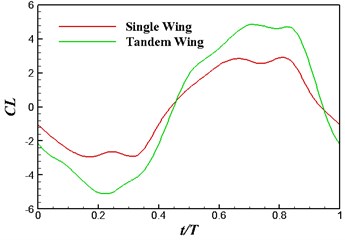
a) Lift coefficient

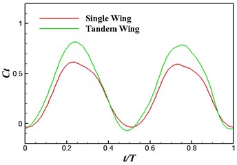
b) Thrust coefficient

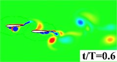
Fig. 5 plots the historical lift and thrust coefficients in one flapping period. It can be seen from the figure that both the $C L$ and $C t$ have a notable increase when the flapping wing is combined with a rearward tail. The computational results, hence, evidence that the aerodynamic interaction between the flapping wing and the tail has a beneficial effect on the propulsive performance. In order to provide a detailed insight into the wing-tail interaction, the vorticity contours of the three flapping configurations are plotted in Fig. 6. In the three flapping modes, similar flow topology of the forward flapping wing(s) can be observed. When the tail is present in the flow field, a leading edge vortex forms on the tail during the down stroke of the forward flapping wing, seen in Fig. 6 middle column, which converts the vertical energy generated by the flapping wing into additional lift and thrust. It is also noted that at $t / T =$ 0.9, the leading edge vortex shed from the forward flapping wing directly blows the stationary leading edge on the tail, which causes a dramatic drop of $C L$ and $C t$ in Fig. 5. For the biplane model, seen in Fig. 6 (right column), the flow performance behaves extremely unsteady due to opposed motion of the oscillating airfoils.

Fig. 6Vorticity contour in half period

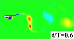
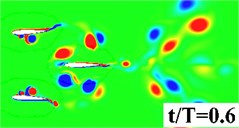
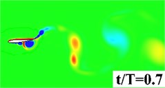
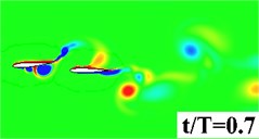
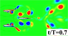
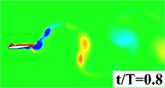
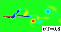
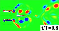
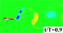
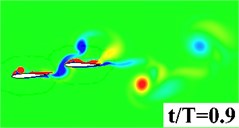
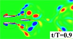
a) Single wing

b) Tandem Wing

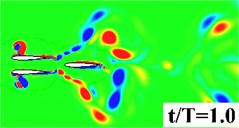
c) Biplane Wing

5.2. Effect of flapping frequency

The flapping frequency as a further critical parameter in flapping motion is considered in the present section. Fig. 7 shows the thrust and power coefficients, as well as the efficiency, versus the reduced frequency. As observed in Fig. 6 the thrust and lift of every mode increase nonlinearly when increasing the reduced frequency and the maximal propulsive efficiency occurs around $k =$ 1.0. Note that the maximum efficiency for the single wing is shifted slightly to a lower reduced frequency compared with the wings combined with stationary tail. Fig. 7 also indicates that at low reduced frequencies (say below $k =$ 1.0) the propulsive efficiency of the tandem and biplane configurations is less than that of a single wing as the tail experiences drag. The force due to the tail is significantly dominated by drag.

5.3. Effect of angle of attack

Previous study focuses on the effect of frequency, while for a real ornithopter, it is crucial to fly with an angle of attack to provide net lift during each flapping cycle. In this section we investigate the dynamic performance of angle of attack on single, tandem and biplane configurations. Computation is conducted from AOA = 0° to 20° with an increment of 2.5°. Lift, thrust, power coefficients and propulsive efficiency are plotted in Fig. 8. It can be seen that lift coefficients are increasing with the increasing AOA, and the wing to tail interaction contributes the lift generation. The lift difference between single and tandem models descents after around AOA = 10°, which indicates that the effect of wing to tail interaction become smaller with a higher AOA. Biplane model provides the largest lift in the high angles of attack regime (AOA > 10°), because the lift is integrated on two wings. As seen, the biplane model owns the largest critical AOA around 12.5° from thrust to drag. The propulsive power doesn’t change too much along with the AOA. It is also noted that tandem model has a notable efficiency with small AOA while biplane model can provide a relatively stable propulsive efficiency in a wider AOA range.

Fig. 7Propulsive coefficients versus flapping frequency

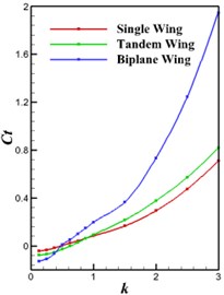
a) Thrust coefficient

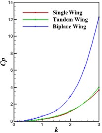
b) Power coefficient

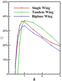
c) Propulsive efficiency

Fig. 8Aerodynamic performance under different AOA of three modes

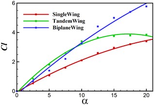
a) Lift coefficients versus AOA

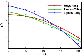
b) Thrust coefficients versus AOA

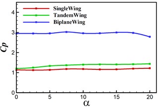
c) Power coefficients versus AOA

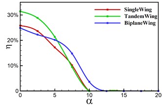
d) Propulsive efficiency

5.4. Effect of wing to tail distance

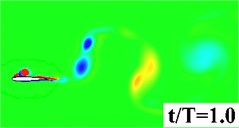
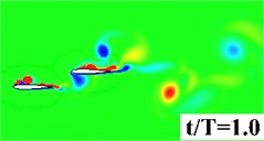
In this section, simulations are conducted to investigate the distance effect between the forward wing and tail. The distance to chord length ratio $L / c$ is set from 0.25 to 2. AOA = 0°, $k =$ 2 are specified for all computations. Fig. 9 gives the vorticity contour of the tandem and biplane models with increasing $L / c$ at $t / T =$ 0.9. It can be seen that a stronger interaction happens when the tail settled closer to the forward flapping wing. Leading edge vortex on the tail can be obviously found when $L / c$ is smaller than 1.0. In order to provide a detailed insight for the propulsive performance, $C t$ , $C_{P}$ and the propulsive efficiency versus $L / c$ of tandem and biplane models, respectively, are plotted in Fig. 10. It is noted that $C t$ and $C p$ decrease with the increasing wing to tail distance; therefore, it can conclude that the wing to tail interaction contributes more thrust when $L / c$ is smaller. In Fig. 10(b) the change in biplane model is too small that can be omitted when compared to tandem model. The radio of thrust generated by tail to the total thrust is shown in Fig. 11. The lift contribute by tail can peak to around 30 % for tandem mode, while only drag is produced on the tail when the tail is mounted behind a symmetrical biplane configuration when AOA = 0°.

Fig. 9Vorticity contour with different wing to tail distance

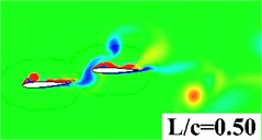
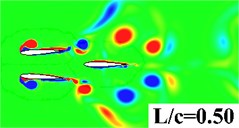
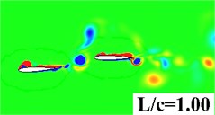
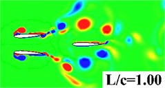
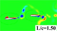
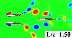
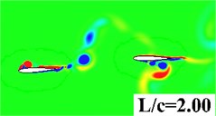
a) Tandem model

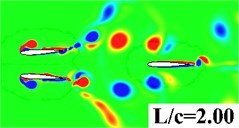
b) Biplane model

Fig. 10Aerodynamic performance under different wing to tail distance

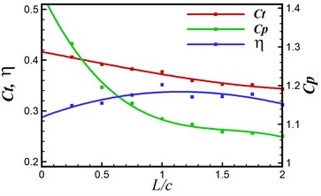
a) Tandem model

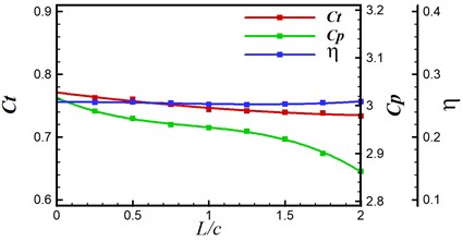
b) Biplane model

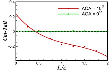
It is known that the tail in the biplane mode can only give negative effect at least when AOA = 0°, however, the biplane configuration employed by real ornithopters such as DelFly use their tails mounted with rudder and elevator for directional and longitudinal operation. In order to investigate the control performance of tail for biplane mode, moment behavior on tail with different wing to tail distances for a given AOA = 10° is shown in Fig. 12, moment center locates at the leading edge of the oscillating airfoils. The period averaged moment coefficients for AOA = 0° are all located at about 0, which illustrates that the tail is not functional when the ornithopter flies at AOA = 0°. However, when applied with AOA = 10°, the tail can provide a reliable control moment and the control moment decreases with the increasing wing to tail distance. Such conclusion has been proved on the real DelFly flapping wing MAV that it is easy to control the flapper when the tail closely mounted behind the forward wing.

Fig. 11Ratio of tail thrust to the total thrust of tandem and biplane modes

Fig. 12Moment coefficient under AOA = 0° and 10°

6. Conclusions

The propulsive characteristics of three different flapping models: single wing, tandem wings, and biplane wings are numerically simulated by a URANS solver coupled with an overset grid method. Effect of oscillating frequency, angle of attack and wing to tail distance are detailed investigated. The wing-tail interaction significantly benefits the thrust generation when the wings are tandem arranged. Moreover, tandem wing is the most efficiency model when applied with high frequencies. Biplane wings model has the most inefficiency propulsive performance, nevertheless it can provide enough thrust force. With the increasing AOA, biplane has the largest critical angle from thrust to drag. Wing-tail interaction becomes weaker when the tail is mounted further from the flapping wings. The present of the tail in tandem model bring more benefits compared with the tail in biplane model. The tail in biplane model is only functional for flight control when applied with a non-zero angle of attack.

References

Knoller R. Die gesete des luftwiderstandes. Flug und Motortechnik, Vol. 3, 21, p. 1-7, (in German).

Search CrossRef
Betz A. Ein Beitrag zur Erklaerung des Segefluges. Zeitschrift fuer Flugtechnik und Motorluftschiffahrt, Vol. 3, 1912, p. 269-272, (in German).

Search CrossRef
Katzmayr R. Effect of Periodic Changes of Angle of Attack on Behaviour of Airfoils, NACA Report (Translated from Zeitschrift fur Flugtechnik and Motorluftschiffahrt), 1922, p. 80-82+95-101

Search CrossRef
Garrick L. E. Propulsion of a Flapping and Oscillating Airfoil, NACA Report, Vol. 567, 1936.

Search CrossRef
Von Karman T., Burgers J. M. General Aerodynamic Theory-Perfect Fluids, Aerodynamic Theory. Julius-Springer, Berlin, 1943.

Search CrossRef
Deng S., Percin M., van Oudheusden B. Experimental investigation of aerodynamics of flapping-wing micro-air-vehicle by force and flow-field measurement. AIAA Journal, Vol. 54, Issue 2, 2016, p. 588-602.

Publisher
Deng S., van Oudheusden B. Wake structure visulization of a flapping-wing micro-air-vehicle in forward flight. Aerospace Science and Technology, Vol. 50, 2016, p. 204-211.

Publisher
Deng S., Xiao T., van Oudheusden B., Bijl H. A dynamic mesh strategy applied to the simulation of flapping wings. International Journal for Numerical Methods in Engineering, 10.1002/nme.5160, 2016.

Publisher
Weiss J. M., Smith W. A. Preconditioning applied to variable and constant density flows. AIAA Journal, Vol. 33, Issue 11, 1995, p. 2050-2057.

Publisher
Xiao T., Ang H., Yu S. A preconditioned dual time-stepping procedure coupled with matrix-free LU-SGS scheme for unsteady low speed viscous flows with moving objects. International Journal of Computational Fluid Dynamics, Vol. 21, Issues 3-4, 2007, p. 165-173.

Publisher
Tuncer I. H., Kaya M. Thrust generation caused by flapping airfoils in a biplane configuration. Journal of Aircraft, Vol. 40, Issue 3, 2003, p. 509-515.

Publisher
Miao J. M., Ho M. H. Effect of flexure on aerodynamic propulsive efficiency of flapping flexible airfoil. Journal of Fluids and Structures, Vol. 20, 2006, p. 401-419.

Publisher
Anderson J. M., Streitlien K., Barrett D. S., Triantafyllou M. S. Oscillating foils of high propulsive efficiency. Journal of Fluid Mechanics, Vol. 360, Issue 360, 1998, p. 41-72.

Publisher
Taylor G. K. Flying and swimming animals cruise at a Strouhal number tuned for high power efficiency. Nature, Vol. 425, 2003, p. 707-711.

Publisher

Cited by

2023 Asia-Pacific International Symposium on Aerospace Technology (APISAT 2023) Proceedings

Kai Wang | Long Chen | Yanlai Zhang | Jianghao Wu

(2024)

Propulsive performance of plunging airfoils in biplane configuration

S. B. Yucel | M. Sahin | M. F. Unal

(2022)

Numerical study of the sound generated by two tandem arranged wings in forward flight

Nathan A Widdup | Li Wang | Fang-Bao Tian

(2021)

Experimental investigations of different fiber orientations on damping loss factor of fiberglass composite specimens

A.V. Borgaonkar | M.B. Mandale | V.G. Salunkhe | S.B. Potdar

(2020)

Effect of Wing-Wing Interaction on the Propulsive Performance of Two Flapping Wings at Biplane Configuration

Jianyang Zhu | Bin Lei

(2018)

Numerical investigation on the propulsive performance of flexible flapping fins using CFD/CSD method

Long Liu | Haisong Ang

(2017)

About this article

Received

18 October 2015

Accepted

18 January 2016

Published

15 May 2016

SUBJECTS

Flow induced structural vibrations

DOI

https://doi.org/10.21595/jve.2016.16568

Keywords

flapping wings

single

tandem

biplane

aerodynamic performance

This is an open access article distributed under the Creative Commons Attribution License, which permits unrestricted use, distribution, and reproduction in any medium, provided the original work is properly cited.

Previous article in issue Previous Next article in issue Next

Research article

2017 09 30

Numerical investigation and experimental test on aerodynamic noises of the bionic rear view mirror in vehicles

Jing Wan, Lei Ma

Research article

2017 08 15

Numerical simulation and experimental research on aerodynamic noises of the single wheel landing gear in an aircraft

Yao-ming Zhou, Yao-long Liu, Shao-wei Li, Dao-chun Li, Yu-hong Jia

Research article

2017 03 31

Numerical investigation on the propulsive performance of flexible flapping fins using CFD/CSD method

Long Liu, Haisong Ang

Research article

2016 12 31

Numerical computation of aerodynamic noise of two tandem circular cylinders and flapping wing motion based on immersed boundary method

Zhi-jun Meng, Yao-ming Zhou, Dao-chun Li

Y. Shen and H. Cai, “Aerodynamic characteristics of multiple flapping wing configurations,” Journal of Vibroengineering, Vol. 18, No. 3, pp. 1839–1848, May 2016, https://doi.org/10.21595/jve.2016.16568

Copy Extrica

Copied to clipboard!

TY  - JOUR
DO  - 10.21595/jve.2016.16568
UR  - https://doi.org/10.21595/jve.2016.16568
TI  - Aerodynamic characteristics of multiple flapping wing configurations
T2  - Journal of Vibroengineering
AU  - Cai, Hongming
AU  - Shen, Yuan
PY  - 2016
DA  - 2016/05/15
PB  - JVE International Ltd.
SP  - 1839-1848
IS  - 3
VL  - 18
SN  - 1392-8716
ER  - 

Copy Ris

Copied to clipboard!

@article{Cai_2016,
	doi = {10.21595/jve.2016.16568},
	url = {https://doi.org/10.21595/jve.2016.16568},
	year = 2016,
	month = {may},
	publisher = {{JVE} International Ltd.},
	volume = {18},
	number = {3},
	pages = {1839--1848},
	author = {Hongming Cai and Yuan Shen},
	title = {Aerodynamic characteristics of multiple flapping wing configurations},
	journal = {Journal of Vibroengineering}
}

Copy Bibtex

Copied to clipboard!

[1]H. Cai and Y. Shen, “Aerodynamic characteristics of multiple flapping wing configurations,” Journal of Vibroengineering, vol. 18, no. 3, pp. 1839–1848, May 2016, doi: 10.21595/jve.2016.16568.

Copy IEEE

Copied to clipboard!

Cai, Hongming, and Yuan Shen. “Aerodynamic Characteristics of Multiple Flapping Wing Configurations.” Journal of Vibroengineering 18, no. 3 (May 15, 2016): 1839–48. https://doi.org/10.21595/jve.2016.16568.

Copy Chicago

Copied to clipboard!

Aerodynamic characteristics of multiple flapping wing configurations

Abstract

1. Introduction

2. Numerical methodology

2.1. Arbitrary Lagrangian Eulerian Navier-Stroke equations

2.2. Aerodynamic force and power calculation

3. Solver verification and validation

4. Flapping wing kinematics and computational set-up

5. Results and discussions

5.1. Effect of wing to tail interaction

5.2. Effect of flapping frequency

5.3. Effect of angle of attack

5.4. Effect of wing to tail distance

6. Conclusions

References

Cited by

About this article

Related Articles