Numerical computation of aerodynamic noise of two tandem circular cylinders and flapping wing motion based on immersed boundary method

2.1. Governing equation

In this paper, the hybrid method based on hydrodynamic force/acoustic separation [32, 33] is adopted to directly compute aerodynamic noise under low Mach number. With this method, all flow variables can be decomposed into incompressible parts and compressible perturbation parts as follows:

Governing equations for incompressible parts are incompressible N-S equation (INS), which represents flow information. Acoustic pulsation and the other compressible effects can be expressed by perturbation variable; the incompressible N-S equation is written in the following:

After obtaining the incompressible flow solution, acoustic perturbation variables can be obtained by solving linearized acoustic perturbation compressible equation (LPCE) [34]. The vector of LPCE equation set can be written as follows:

where $s\mathrm{\text{'}}$ is any additional prescribed acoustic source. The boundary conditions on the solid wall are as follows:

where $\widehat{n}$ is the unit wall-normal vector, and the initial conditions are normally $\rho \mathrm{\text{'}}=\overrightarrow{u\mathrm{\text{'}}}=0$ and $p\mathrm{\text{'}}={p\mathrm{\text{'}}}_0$. Furthermore, the perturbed velocity (Eq. (5)) and pressure (Eq. (6)) fields are decoupled from the perturbed density field (Eq. (4)), and if one is not interested in a perturbed density field, this equation does not need to be solved. The left hand sides of LPCE represents the effects of acoustic wave propagation and refraction in the unsteady, inhomogeneous base flows, while the right hand side only contains the acoustic source term. For low-Mach number flows, it is interesting to note that the total change of hydrodynamic pressure $DP/Dt$ is the only source term coming from the incompressible base flow and this is consistent with the analysis of Goldstein [36]. The LPCE have been well validated for fundamental dipole/quadruple flow noise problems [37] and also for the low-Mach number turbulent flow noise problems [34, 38]. Further details regarding the derivation of LPCE can be found in Reference [37].

2.2. Numerical method

Incompressible N-S Eq. (3) is solved by one and one step. The spatial derivatives are obtained by using two order central differences. And the flow items and dissipation items are subject to time integral by means of two-order Adams-Bashforth method and Crank-Nicolson method. Pressure Poisson equation is solved by means of multiple mesh method. LPCE spatial discretization is subject to six-order compact central difference, and time integral is subject to four-order Runge-Kutta. Three-order and four-order boundary schemes are adopted near the immersed solid boundary and the computing domain boundary. Because there is no dissipation error in compact central difference, implicit spatial filtering is adopted to restrain high frequency errors for the purpose of ensuring numerical stability. In this paper, ten-order filtering is adopted in the internal areas, and the filtering near the boundaries reduces to two-order from eight-order successively. Compact central difference and the filtering of implicit spatial can be solved by means of tridiagonal matrix.

2.3. Immersed boundary method

The flow problems which have complex immersed boundaries can be completed by the incompressible N-S equation [30]. Before integral for the governing equation, all the elements inside the object are marked as “body point”, and other points outside the object are marked as “fluid point”. Any “body point” adjacent to fluid point is marked as “image point”, as shown in Fig. 1(a). Wall boundary conditions are realized by setting proper values for the image point. In the method of Mittal [30], an “orthogonal” extends to the immersed boundary from the image point. The probe continues extending to the body reaching the “ghost point”, so as to locate the object point at a middle position between the image point and the ghost point. The value of the image point can be computed through linear interpolation by the values of the boundary point and the ghost point along the orthogonal probe direction. The value of the ghost point is obtained through three-dimensional three-linear interpolation by the surrounding fluid points. This provides the boundary conditions of the immersed boundary with the feature of nominal second order accuracy.

Image point value determines whether the boundary conditions at the object point (BI) is met. In particular, a general variable $\varphi$ is used for estimating with $N$-order polynomial $\mathrm{\Phi }$ near object points $(x_{BI},y_{BI},z_{BI})$:

In the above equation, $x\mathrm{\text{'}}=x-x_{BI}$, $y\mathrm{\text{'}}=y-y_{BI}$, $z\mathrm{\text{'}}=z-z_{BI}$, $c_{ijk}$ is an unknown coefficient and is expressed as follows:

Fig. 1Diagram of image elements and boundary conditions

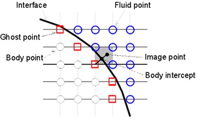
a) Diagram of image elements

b) Diagram of boundary conditions

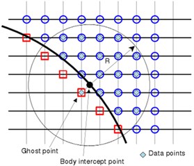
The size of coefficients for three-order polynomial ($N=$3) is 10 and 20 under two-dimensional and three-dimensional conditions, respectively. To determine these coefficients, the data of the flow field points around the object needs to be obtained. According to the method of Luo [35], the flow field points in the circle or ball (under three-dimensional conditions) with the object point as the center and the radius of $R$ can be selected. For $M$ data points, coefficient $c_{ijk}$ is determined by minimum weighted error estimation:

where $w_m^{}$ is the weight function. According to the previous research experience [35], cosine weight function is used in this paper. To make the least square problem appropriate, radius $R$ should be selected in a way which can ensure that there are more data points than coefficients. To find the values of the image point and the object point, the first data point is selected as image points, other ($M-$1) data points shall be found in the fluid region (as shown in Fig. 1(b)). The accurate solution of least square problem (Eq. (10)) is as follows:

wherein, the superscript + represents generalized inverse of the matrix, vector$\mathrm{c}$and $\varphi$ include coefficient $c_{ijk}$ and data $\varphi (x_m^{\text{'}},y_m^{\text{'}},z_m^{\text{'}})$ respectively; $\mathbf{W}$ and $\mathbf{V}$ indicate weight matrix and Vandermonde matrix respectively. It’s noteworthy that $(x_1^{\text{'}},y_1^{\text{'}},z_1^{\text{'}})$ represents image points. After solving Eq. (11), coefficient $c_{i\mathrm{j}k}$ can be written as the linear combination of $\varphi (x_m^{\text{'}},y_m^{\text{'}},z_m^{\text{'}})$. According to Eq. (9), coefficient $c_{ijk}$ represents the value and derivative value of $(x_{BI},y_{BI},z_{BI})$:

Therefore, for the Dirichlet and Neumann boundary conditions given on object wall, the image point values can be obtained by Eq. (11) and Eq. (12).

Fig. 2Diagram of moving boundary and updated elements

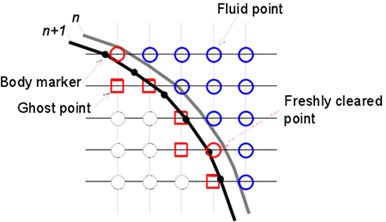
a) Diagram of moving boundary

b) Diagram of updated elements

2.4. Disposal for the updated elements

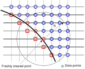
Arbitrary movement of the object is realized by describing the displacement of each node (object identification point) on the triangular mesh of the surface for the immersed object. Disposing the moving object on the fixed mesh will generate “updated elements”, as shown in Fig. 2(a). As the time-dependent variable values of the updated elements don’t need to participate in integral of the governing equation, it is only obtained by the adjacent elements through interpolation [35]. During solving the incompressible flow, the variable values of the new time layer are obtained by iterations of three times of linear interpolation together with the solution of the momentum equation[30]. During solving acoustics, the values of the updated elements are obtained through high order approaching multinomial. The entire process is similar to the disposal for image elements in Section 2.3. However, for the updated element, the center of the data points is updated element $(x_{FC},y_{FC},z_{FC})$, where $x\mathrm{\text{'}}=x-x_{FC}$, $y\mathrm{\text{'}}=y-y_{FC}$, $z\mathrm{\text{'}}=z-z_{FC}$, as shown in Fig. 2(b). To avoid iterations, only the non-updated elements and fluid elements are selected as the data points to minimize Least Squares Error. The coefficient of the approaching multinomial will be obtained by solving Eq. (11), and then the value of the updated element can be directly given by the first coefficient, for instance:

3.1. Turbulent flow noises of two tandem circular cylinders and experimental verification

Two tandem circular cylinders are used as the research object in the paper. Its model is established for numerical simulation, so as to investigate the flow field and flow noise of the fluid when it passes through two tandem circular cylinders. The physical model depended by the numerical simulation can be found in Fig. 3. In the model, the origin of coordinates is located in the center of the upstream cylinder. $L/D$ is an important parameter, wherein $D$ is the cylinder diameter and L represents the center distance of two cylinders. The center of the upstream cylinder is at a distance of 5$D$ from the inlet surface, three inlet boundary conditions of speed are given and one outlet boundary condition of pressure is supposed. The circumferential flow field of two circular cylinders is computed by the immersed boundary method and the acoustic field is also computed. To facilitate noise analysis, fast Fourier transform is used to transform fluctuating pressure under time domain into that under frequency domain.

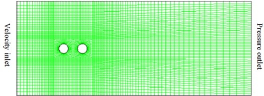
Details of turbulent flow, especially the details of fluctuating turbulent flow, can be captured through finer meshes, which is very important for solving noises. To improve the computational accuracy, the structured mesh is divided to 18 computational zones, as shown in Fig. 4. The encryption was made for the vicinity of cylinder wall, the wake and other regions with relatively complex structures. Considering the computational efficiency brought forward from the fine degree of the meshes, the distance between the wall surface and the first layer of meshes was set as 0.012 mm and then increased externally in proportion. Inflow velocity is $U_0=\mathrm{}$44 m/s and corresponding Reynolds number is $R{e}_D=$ 1.66×10⁵. Mach number is $M=$ 0.128. The size of computation domain is $-\text{40}D\le x\le \text{200}D$, $-\text{30}D\le y\le 30D$. Span-wise length is $L_z=3D$. The total number of non-uniform Cartesian meshes is 768×384×32.

Boundary conditions have to be chosen carefully in order to obtain results which are consistent with physical properties. This paper takes flow velocity as known conditions to compute the turbulent flow noise of two tandem circular cylinders. Therefore, inlet boundary chooses velocity inlet boundary conditions. In the meanwhile, velocity inlet boundary conditions are selected and used for the upper and lower parts of the computational domain. Outlet boundary is pressure outlet boundary. Other boundaries choose wall boundary conditions. The circumferential flow field of two tandem circular cylinders is extremely complex, and the details of the flow should be captured as much as possible during computing noises, so small time steps must be chosen. Meanwhile, considering the restrictions of noise frequency from time step, the interested frequency is less than 5000 Hz, and the time step is 0.0001 s finally.

Fig. 3Physical model of two tandem circular cylinders

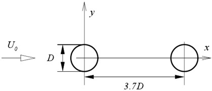
Fig. 4Diagram of computational meshes for two tandem circular cylinders

Based on the above computational model, the pressure factor of circumferential flow field for two tandem circular cylinders could be obtained, as shown in Fig. 5. In the figure, BART and QFF represent experiments made by Basic Aerodynamics Research Tunnel and Quiet Flow Facility in NASA center, respectively. As can be seen from Fig. 5(a), the pressure coefficients of upstream and downstream cylinders computed herein show a good consistency with that of the experimental results, but a large deviation between simulation and test is appeared in a few angles, which is within the acceptable range. This indicates the effectiveness of the numerical model in this paper.

The contour of vorticity distribution of two tandem circular cylinders can be found in Fig. 6. It is indicated that the flow process is very complex due to the coupling existing between two tandem circular cylinders. In addition, the separation of flow shear layer is appeared in the upper layer of the upstream cylinder, forming a vortex structure. The upstream cylinder has shown the rolling state of wake before reaching the downstream cylinder, and then its vortex shedding interacts with that of the downstream cylinder. According to Howe’s vortex shedding theory, the aerodynamic noise is caused precisely by vortex shedding.

Fig. 5Comparisons of pressure coefficient for two tandem circular cylinders

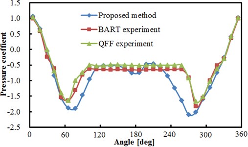
a) Comparisons between experiment and simualtion for upstream cylinder

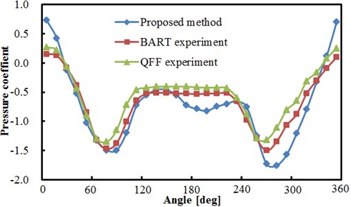
b) Comparisons between experiment and simulation for downstream cylinder

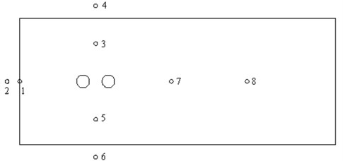
A certain direction is generally shown in noise radiation. To compare the similarities and differences in all directions of perturbation noise of two tandem circular cylinders, eight observation points were defined around the computational model to receive the sound pressure signal, as shown in Fig. 7. In the figure, observation points 1, 4 and 6 are of the same distance to the center of two tandem circular cylinders. Observation points 3, 4, 5 and 6 are in the vertical plane, while observation points 1, 2, 7 and 8 are in a horizontal plane. According to the above computation result and model, the sound field can be further computed in Fluent, whose results are shown in Fig. 8.

The comparison result of sound pressure levels in observation points 3 and 4 is shown in Fig. 8(a), and two observation points are in the same direction and plane. As can be seen from the figure, the sound pressure level of observation point 3 is significantly greater than that of point 4 over the entire frequency domain, with the biggest difference of nearly 50 dB. The maximum sound pressure level of observation point 3 is 117.2 dB appearing at the frequency near 352 Hz. The maximum sound pressure level of observation point 4 is 100 dB appearing at the frequency near 352 Hz. At the frequency below 2000 Hz, the sound pressure level of observation points 3 and 4 is generally decreased gradually along with the increasing frequency. At the frequency above 2000 Hz, the sound pressure level of observation points 3 and 4 tends to be stabilized generally, which only fluctuates near a certain value. Throughout the entire frequency domain, the valley points of observation point 4 are significantly greater than that of point 3.

Fig. 6Contour of vorticity distribution for two tandem circular cylinders

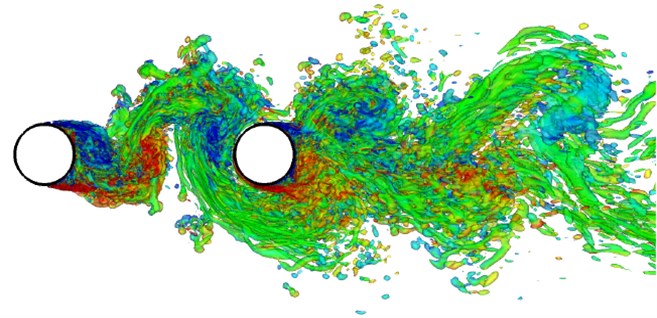
Fig. 7Observation point position of sound pressure signal

The comparison result of sound pressure levels in observation points 1 and 4 is shown in Fig. 8(b), and two observation points in different planes are of the same distance to the center of two tandem circular cylinders. As can be seen from the figure, the sound pressure level of observation point 4 is significantly greater than that of point 1, with the biggest difference of nearly 40 dB. It is indicated that the radiation noise of two tandem circular cylinders has shown obvious directivity, and the radiation noise in the vertical direction is greater than that in the horizontal direction. The maximum sound pressure levels of observation points 1 and 4 are 88.5 dB and 100 dB, respectively, both appearing at the frequency near 352 Hz. In the entire frequency domain, the valley values of observation point 1 are significantly greater than that of point 4. At the frequency below 1000 Hz, the fluctuations of sound pressure levels are relatively large with evident peaks and valleys. At the frequency below 2000 Hz, the sound pressure level is generally decreased gradually along with the increasing frequency. At the frequency above 2000 Hz, the sound pressure level of two observation points tends to be stabilized generally, which only fluctuates near a certain value. The comparison results in Fig. 8(c) are similar to Fig. 8(b). As can be seen from Fig. 8(b) and Fig. 8(c), the noise intensity in vertical plane is larger than that in horizontal plane.

Fig. 8Comparison of sound pressure levels at observation points

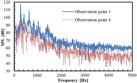
a) Comparison of sound pressure levels in observation points 3 and 4

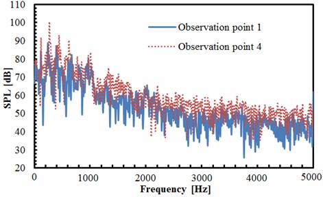
b) Comparison of sound pressure levels in observation points 1 and 4

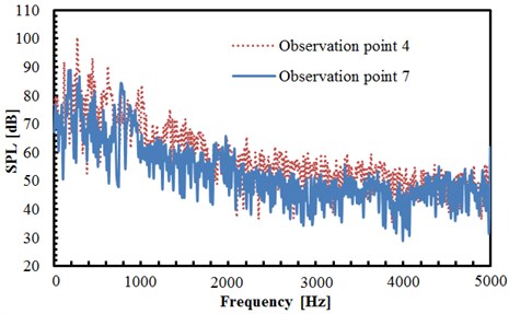
c) Comparison of sound pressure levels in observation points 4 and 7

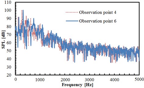
d) Comparison of sound pressure levels in observation points 4 and 6

The comparison result of sound pressure levels in observation points 4 and 6 is shown in Fig. 8(d), and two observation points in the same plane are of the same distance to the center of two tandem circular cylinders. However, the observation point 4 is above the upstream cylinder while point 6 is below the upstream cylinder. As can be seen from the figure, both trends and values of sound pressure levels of two observation points are close, but only peak frequencies of them are slightly different. However, the maximum sound pressure level of both observation points is 100 dB, both appearing at the frequency near 352 Hz. At the frequency below 1000 Hz, the fluctuations of sound pressure levels are relatively large with evident peaks and valleys. At the frequency below 2000 Hz, the sound pressure level is generally decreased gradually along with the increasing frequency. At the frequency above 2000 Hz, the sound pressure level of two observation points tends to be stabilized generally, which only fluctuates near a certain value. In addition, as seen from the analysis of Fig. 8(b) and Fig. 8(c), the acoustic field of two tandem circular cylinders in the vertical plane is distributed symmetrically, and its intensity is larger than that in the horizontal plane.

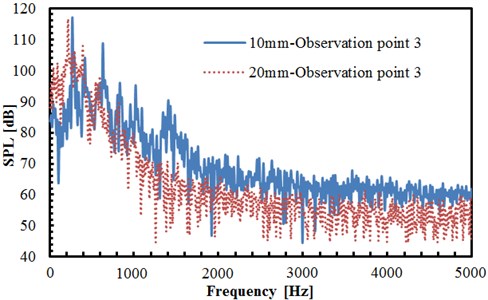
Two tandem circular cylinders analyzed have the diameter of 10 mm. In the above analysis, the ratio of the cylindrical diameter to the distance between two cylinders would have a serious impact on the flow noise. Therefore, the cylindrical diameter is changed to 20 mm, and the acoustic field distribution around the cylinder is observed. The comparison of sound pressure levels of observation points under cylindrical diameters 10 mm and 20 mm can be found in Fig. 9.

The comparison of radiation noises at the observation point 3 under cylindrical diameters 10 mm and 20 mm can be found in Fig. 9(a). As can be seen from the figure, the sound pressure levels of observation points under the cylindrical diameter of 10 mm is significantly greater than that under the diameter of 20 mm. The maximum sound pressure level under the cylindrical diameter of 10 mm is 118 dB and corresponding frequency is 352 Hz. The maximum sound pressure level under the cylindrical diameter of 20 mm is 116 dB and corresponding frequency is 346 Hz. Therefore, maximum sound pressure levels under different cylindrical diameters only have small differences in the analyzed frequency band and corresponding frequencies approximate 352 Hz. The main reason is that results in low frequencies are mainly affected by boundary conditions for acoustics, and boundary conditions analyzed by different cylindrical diameters are basically the same. Before the frequency point of the maximum sound pressure level, the sound pressure level under the cylindrical diameter of 20 mm is greater than that under the diameter of 10 mm. However, when the frequency exceeds the point of the maximum sound pressure level, the sound pressure level under the cylindrical diameter of 10 mm is greater than that under the diameter of 20 mm, which is only different in individual frequency points. It is mainly because the distance between two circular cylinders is 3.7$D$ and the change of cylindrical diameter greatly changes the distance between two circular cylinders. Under the cylindrical diameter of 20 mm, the distance between two circular cylinders increases to 74 mm. Therefore, the noise between two circular cylinders is relatively low. Moreover, at the frequency below 2000 Hz, the sound pressure level of two cylindrical diameters is generally decreased gradually along with the increasing frequency. But at the frequency above 2000 Hz, the sound pressure level tends to be stabilized near a certain value. The acoustic pressure level under the cylindrical diameter of 20 mm has presented obviously more valley value than that under the diameter of 10 mm.

The comparison of radiation noise at the observation point 4 under cylindrical diameters 10 mm and 20 mm can be found in Fig. 9(b). As can be seen from the figure, the trend of the sound pressure level is not similar to that in Fig. 9(a). The sound pressure level corresponding to different cylindrical diameters is generally of little difference. Only at the frequency of 400 Hz, a larger difference between the two cylindrical diameters is shown. In this case, the sound pressure level under the cylindrical diameter of 20 mm is greater than that under the diameter of 10 mm. Furthermore, obviously more valley values are appeared in the sound pressure level under the cylindrical diameter of 20 mm.

Fig. 9Comparison of sound pressure levels of observation points under different cylindrical diameters

a) Comparison of sound pressure levels of observation point 3 under different cylindrical diameters

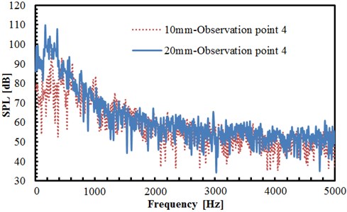
b) Comparison of sound pressure levels of observation point 4 under different cylindrical diameters

3.2. Flow noise induced by flapping wing motion

To verify whether this method is applicable to flow noise problems of moving objects with complex profiles, flapping wing sound generation is computed in this section. Flapping wing is a common structure of insects or micro unmanned aerial vehicle (MAV). Since the micro size of the flapping wing, velocity and Reynolds number are relatively small, and the aerodynamic properties at this time are different from that under the high Reynolds number. Its wing boundary layer becomes sensitive to the changes of the angle. And the separation of its wing boundary layer would be even caused by the minor changes, forming laminar separation bubbles, deteriorating aerodynamic characteristics of wing and appearing increased resistance, significantly dropping the lift to drag ratio and other adverse effects. Along with the flapping of the wing, the surrounding flow field makes unsteady flow, which is therefore difficult to give an accurate explanation by the conventional aerodynamic method. Fig. 10 is the diagram for flapping wing problem. The main body and the wing are standard geometric models, including the wing length of c, the airframe of 0.5$c$ and the wing width of 0.4$c$. The angular velocity of flapping wing movement is described by sine function:

wherein, $V_{\mathrm{m}\mathrm{a}\mathrm{x}}$ is the maximum speed at wing-tip, $r_{tip}=\text{1.5}c$ is the distance from the body center to the wing-tip, $T$ is the period. Wing length $c$ and the maximum speed $V_{\mathrm{m}\mathrm{a}\mathrm{x}}$ of wing-tip are selected as the characteristic scales of length and speed. The left and right wings move symmetrically in since function manner. The Reynolds number is 200, Strouhal number is $c/T{V}_{\mathrm{m}\mathrm{a}\mathrm{x}}=$ 0.25, Mach number based on wing-tip speed is $M=$ 0.1. The number of Cartesian grid is 512×512, of which wing length $c$ is distinguished by 60 meshes, as shown in Fig. 11(a). See Fig. 11(b) for the contour of vorticity of instantaneous flow field. (as known from the figure, the wingtip has a relatively large speed, showing complementary and symmetrical structure, which is mainly because the wing and airframe are symmetrical and make sinusoidal movement.) Curve of lift coefficient of wing and airframe changing with time is as shown in Fig. 12. (lift coefficient is changed in the similar periodicity to flapping wing movement.) Because of symmetry, the left and right wings share the same lift coefficient. The changing of airframe lift coefficient is caused by the fluid induced by flapping wing movement, (airframe lift coefficient is about one half of the wing, which is consistent with the sizes of airframe and wing).

Fig. 10Diagram of flapping wing motion model

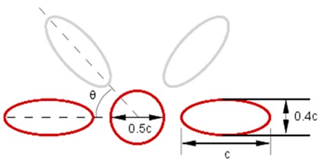
Fig. 11Computational domain of flapping wing movement and contour map of vorticity

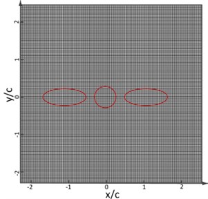
a) Diagram of flapping wing motion model

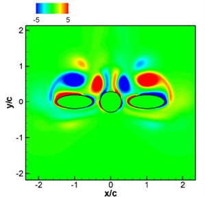
b) Contour map of the instantaneous vorticity

Fig. 12Curve of lift coefficient of flapping wing model with time

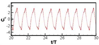
a) Wing of flapping wing model

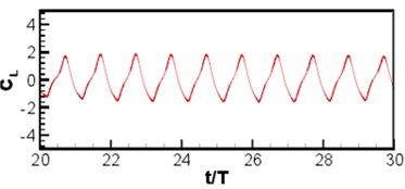
b) Airframe of flapping wing model

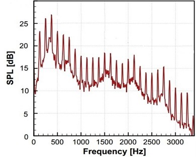
The instantaneous diagram for acoustic field computed by LPCE is as shown in Fig. 13(a). (Because of symmetry, the left and right wings have the same acoustic field.) Based on Strouhal number and Mach number, the wavelength of the main wave is 40$c$. Symmetric flapping wing movement is similar to dipole source, and the sound directivity is shown in Fig. 13(b) where a dipole source can be seen in longitudinal direction. Curves of acoustic pressure changing with time monitored at point (0, 60$c$) and (0, –60$c$)are as shown in Fig. 14. The signal changes periodically, the sound pressure signal presents a periodic change, and sound pressure changes of the symmetrical two observation points are not exactly consistent with a certain phase difference. Although the geometrical shape and movement of the computational model are simple, the computational results show that the algorithm can distinguish the sound generation problems of moving objects very well. To further investigate the sound pressure characteristics of aerodynamic noises, the sound pressure level spectrum of flapping wing motion at different frequencies is shown in Fig. 15. As can be seen from Fig. 15, the interval of peaks in sound pressure level curve is basically remained the same, and the sound pressure level is gradually decreased along with the increasing frequency. The maximum sound pressure level is 26 dB appearing at the frequency near 400 Hz.

Fig. 13Computational results of acoustics for flapping wing model

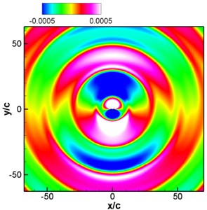
a) Contour of instantaneous sound pressure of the flapping wing model

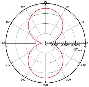
b) Sound directivity pattern ($r=\text{50}c$)

Fig. 14Time domain acoustic pressure at observation points of flapping wing model

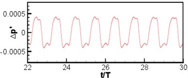
a) (0, 60$c$)

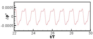
b) (0, –60$c$)

Fig. 15SPL spectrum at different frequencies