Abstract
The flow field distribution characteristics of side windshields and full windshields installed in the connection section of a high-speed train were numerically computed to reduce the aerodynamic noise and improve operating environment of the high-speed train. As shown from the result, the maximum pressure was at the nose tip of the high-speed train; and the greatest flow velocity of fluid was centered in the middle section of the body, while the flow velocity at both ends of the body was relatively small. After installing a side windshield, the fluid pressure of the side was significantly lower than the upper and lower surfaces, and the pressure and turbulence intensity were greater at the corner of the connection section steps. The fluid flowed to the steps from the roof of the train, and then spread gradually down along the side, with the decreasing flow rate. Therefore, the airflow was effectively prohibited from flowing into the train through installing side windshields. However, after further installing full windshields, the pressure, flow velocity and turbulence intensity in the connection section of the high-speed train were further improved. Then, the boundary element method was applied to compute the radiation noises of two kinds of windshields installed in the connection section of the high-speed train. As shown from the result, broadband radiation noise was in the upper connection section, the maximum sound pressure level (SPL) value was between 50-100 Hz and some directivity of sound pressure was shown in the high-frequency range. A certain periodicity of sound pressure distribution was presented in the longitudinal symmetrical plane of the high-speed train. At the same observation point, the sound pressure level of full windshield was slightly reduced at most frequency points, and the maximum reduction value was 23.6 dB. Finally, the wind tunnel test was conducted on the high-speed train, and the connection section of the high-speed train was the obvious noise source, thus indicating that the research in the paper was very meaningful. Besides, from SPL comparisons of the observation point, experiments and simulations were consistent with each other whether side windshields or full windshields were installed in the connection section. As a result, the reliability of the numerical computational model and the effectiveness of the results and analysis were verified.
1. Introduction
If the driving speed of the high-speed train is continuously improved, the aerodynamic noise would be more and more severe or even occupy a more dominant position [1]. Psychological health of passengers and people along the railway would be seriously affected, the fatigue damage of full buildings and related equipment would be caused and their service lives would be shortened by excessive noise. Therefore, train noise pollution has become a bottleneck that constrains the development of the high-speed railway. As shown from studies, the aerodynamic noise of the high-speed train is increased along with the sixth power of the train speed, while power system noises, wheel-rail noises and other mechanical noises only increased with the first power and third power of the train sped [2-4]. Currently, the driving speed of the high-speed train was more than 250 km/h, and the aerodynamic noise is gradually playing a dominant role among all noises with the growth rate of the train speed, thus affecting the ride comfort and environment along the railway. Therefore, researches on aerodynamic noises of the high-speed train and proposing proposal of feasible noise reduction have become the key to control the high-speed train noise [5]. The aerodynamic noise in different positions of the high-speed train has been tested by many scholars. Through low-noise wind tunnel, the impact of apron board and grille of the high-speed train on the noise of both sides of the railway was studied by Frid [6]. The design theory and method of the pantograph with low aerodynamic noise were introduced and the improvement design for its aerodynamic noise was proposed by Ikeda and Iwamoto [7-10]. The aerodynamic noise generated at the door was studied by Sassa through experiments and numerical computations [11]. And the aerodynamic noise of the high-speed train cabin was predicted by Xiao through numerical simulation, with good results achieved by them [12].
However, the above researches were mainly aimed at heads, bogies, wheels and other sections with prominent structures in the high-speed train, not any published paper has been made currently concerning radiation noise in the connection section of two trains. And as shown from the noise source identification results in the paper, the connection section of trains is indeed an obvious noise source. Therefore, the study in the paper is very meaningful.
Large eddy simulation was firstly applied in the paper to study the flow field distribution of a high-speed train with side windshields and full windshields, respectively. Then, the boundary element method was employed to compute its radiation noise, and then a detailed analysis and discussion was conducted, which was made comparison verification with the wind tunnel results.
2. Control equations
2.1. Turbulence model equations
Regarding current simulation of aerodynamic noise, large eddy simulation method is the most desirable method for computing turbulent fluctuation. The large-scale turbulent motion is directly computed by N-S equation in large eddy simulation, while the impact of small-scale vortices on large-scale motion was simulated through building models. Subgrid scale model was introduced in the paper to build N-S equation of large eddy simulation [13-15] as follows:
where is fluid density. is turbulent viscosity coefficient, and referred to subgrid scale stress that reflected the impact of the motion of small-scale vortices on motion equations, whose mathematical model was as follows:
wherein: is the tensor of deformation rate, is the turbulent viscosity of subgrid scale, is symbolized Kronecker Delta, and is the stress in the direction of . Closed equations were formed with the continuity equation to solve it numerically.
2.2. Acoustic boundary element equations
Differential equations of the problem were transformed into boundary integral equations through boundary element method (BEM), then a limited number of boundary elements were introduced to disperse integral equations and obtain equations containing unknowns of boundary nodes, and then numerical computation was conducted. Since control equations of the region was transformed by BEM into the integral equations along the regional boundary, only boundary elements were required to be defined and boundary conditions were combined to solve the equations, which could reduce the dimension of the solved problem to be lower and effectively simplify a complex three-dimensional model into two-dimensional model. Compared with three-dimensional finite element model (FEM) with the same complexity, such model was smaller and easier to create, check and process, which could obtain results within a shorter time. However, equations established by boundary element method were featured with dense and generally asymmetrical coefficient matrix, possessing great computational time of matrix element. As infinity condition, could be automatically satisfied by the differential operator utilized by BEM, the method was particularly convenient for problems regarding infinite domain and semi-infinite domain.
When sound waves were entered into the object, if the interaction between fluid and structure was greater, and it must be considered. The radiation noise of the high-speed train computed in the paper was just one of such conditions, which was computed through the acoustic coupling boundary element theory based on combination of FEM and BEM.
Boundary element method was applied to process and solve integral equations. Boundary should be dispersed by the boundary element into many elements and nodes. And sound pressure and normal velocity and global matrix shape function on the node can be used to represent the sound pressure and normal velocity at any point within each element:
wherein: is the global shape function related to sound pressure and normal velocity on nodes of boundary .
In BEM, some nodes with unknown sound pressure and vibration velocity, such as node , namely , were expressed by the following formula:
wherein: both coefficient matrices and were matrices of .
The sound field distribution and structural vibration displacement of coupled BEM were computed simultaneously. Boundary element meshes can be divided into two parts: one part was coupled with the structure, includingnodes, and the other part was involved in the coupling, including nodes . Therefore, the sound pressure and velocity on the boundary element can be written as follows:
wherein: and were shape functions related to nodes and . Since the sound pressure was acted on the structure as a load, the vibration of the structure can also be caused. Therefore, the dynamic equation of this structure could be expressed as below:
wherein: , and are stiffness matrix, damping matrix and mass matrix of the structural finite element model, respectively. is the structural displacement vector. is the external load acted on the structured meshes (excluding sound pressure loads). is the load of sound pressure acted on the structure. And is the coupling matrix of :
wherein: is the number of elements for the coupled structured mesh, is the shape function of the structural mesh, and is the normal vector of an element. The minus sign is the opposite normal direction of elements between structured mesh and boundary element.
For the coupled boundary element method, the nodes of structured meshes should be coincided with the nodes of sound meshes in the coupling surface between the structure and sound. In the coupling surface , the continuity of vibration velocities of structured meshes and sound meshes was in the following relationship with displacement and velocity , namely . And the following relational expression can be obtained:
wherein: is the known displacement, is matrix, and is the matrix, which were defined as follows, respectively:
wherein: is the normal equation of structured meshes, and the minus sign indicates the opposite directions of normal equations of structured mesh and sound meshes. The Eq. (10) is substituted into Eq. (5) to obtain the following formula:
The finite element Eq. (8) and boundary element Eq. (13) of the structure were combined to get the coupled equation of finite element and boundary element for the structure as follows:
The structural load was obtained through the finite element. Then, the above formula could be employed to obtain the acoustic response of the structure at any point.
3. Computational models and boundary conditions
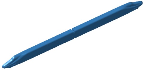
The computational model of the high-speed train was consisted of heads and tails, while the section in the middle was removed. Thus, the size of the computational model could be reduced and the computational time could be improved in the study, as shown in Fig. 1. The connection section between the head and tail was primarily studied in the paper, as shown in Fig. 2. A stepped cavity was formed in the connection section, which would cause the disorder of the airflow in this section and affect the noise distribution around the train.
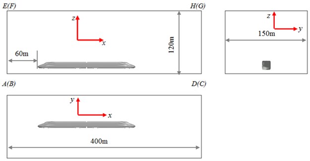
In the numerical simulation, the finite computing domain was generally applied to replace the infinite computing domain. In the length direction of the region, the size was selected so that the downstream boundary of the computational domain could be away from the rear section of the train as far as possible, so as to avoid the impact of wake flow on the outlet section, which was convenient for the definition of outlet boundary conditions. The computational domain and coordinate were defined as Fig. 3. At a constant speed, the boundary conditions of the high-speed train were defined as follows.
The non-slipping boundary condition on the surface could be satisfied by the viscous fluid, which was therefore set on the surface. The slipping boundary condition was set on ground ABCD, the normal velocity was set as zero, and the tangential velocity was consistent with the inflow velocity, in order to eliminate the influence of ground floor. The inlet boundary conditions of the velocity were given on surface ABFE, AEHD and BFGC. At the outlet cross-section, the velocity was 0 indirection, the speed was given different values indirection according to the uniform inflow, and the velocity was 0 in direction. The outlet boundary condition was given pressure on the roof EFGH and surface CDHG, and the outlet static pressure was 0 at the outlet section cross-section.
Fig. 1Computational model of the high-speed train
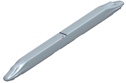
Fig. 2Connection section of the high-speed train
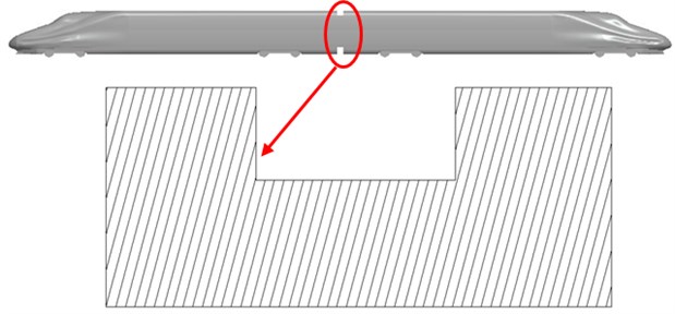
Fig. 3Definition of computational domain and coordinate
4. Numerical computation of flow field around the high-speed train
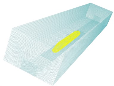
Aerodynamic meshes were divided according to the geometric model of the high-speed train, whose results were shown as Fig. 4. It was shown that very small mesh sizes were applied in the aerodynamic model of the high-speed train, which could ensure higher computational accuracy. A total of 1,023,894 elements and 1,287,369 nodes were included in the aerodynamic model of the high-speed train. Such aerodynamic model and the computational domain in Fig. 3 were chosen as the basis to build the computational model of the high-speed train, as shown in Fig. 5. It could be seen that the computational domain was featured with dense meshes around the high-speed train, and the mesh size was increased gradually along with the rising distance of the high-speed train. Therefore, the computational time was reduced and efficiency was improved, while the flow field distribution around the high-speed train would not be affected.
The structural design in the connection section was not considered enough in current structure of the high-speed train, while the head, bogies and wheels were primarily concerned. The structure in the connection section was attempted to be studied in the paper, and two kinds of windshields were arranged in the connection section to shield the radiation noise and improve the operating environment.
Fig. 4Aerodynamic meshes of the high-speed train
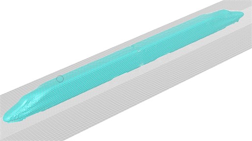
Fig. 5Computational model of flow field for the high-speed train
4.1. Side windshields
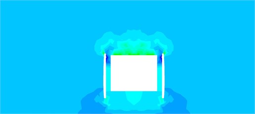
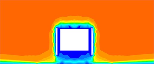
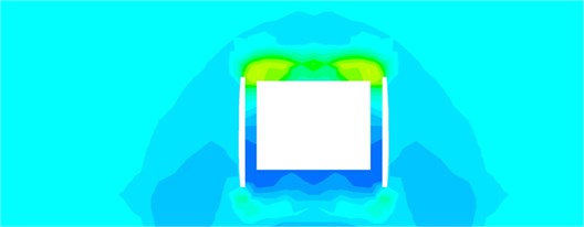
Windshields were only arranged on the sides of the connection section to reduce the structural radiation noise from the connection section to sides. The above numerical model was applied to compute the flow field characteristic in the entire domain of the high-speed train as well as the connection section, whose results were shown in Fig. 6-Fig. 8. It was shown that the flow field characteristic was distributed symmetrically around the high-speed train, and it was because the high speed train was a symmetrical structure. Additionally, the excitation in the simulation was also facing with the longitudinal symmetry plane of the high speed train. When the fluid was flowing backwards from the head, the structural heights contacted by fluid on both sides of the longitudinally symmetrical plane were consistent. Besides, as known from the flow field distribution characteristic of the entire train, maximum pressure was on the nose tip of the high-speed train head; and higher positive pressure could be easily formed in this region due to severe deformation existing in this structure and the bogie, wheels and other complex structural models emerged in the lower section of the train body. Such conclusion was also reflected in turbulence intensity distribution in Fig. 8. As shown from Fig. 7(a), the fluid domain with relatively larger flow velocity was mainly centered on the middle section of the train body, while the relatively small velocity was appeared on both sides of the train body, because severe obstacles in the flow process of the fluid would be caused by the severe structural deformation of both sides of the train body. It was shown from Fig. 6(b) that after installing windshields on the sides of the connection section of the train body, the fluid pressure in the side was significantly lower than that on the upper and lower surfaces. And the fluid pressure and turbulence intensity at the corner of the connection steps were relatively large. It was because windshields can prevent the flow of fluid effectively, and make the fluid pass the top and bottom of the high speed train. It was shown from Fig. 7(b) that the fluid flowed to the connection steps from the upper body, and then gradually diffused along two sides, with the constantly decreasing flow velocity. After installing windshields on both sides, the airflow was effectively prevented from flowing into the train along both sides.
Fig. 6Pressure distribution around the high-speed train

a) Pressure distribution of entire trains
b) Pressure distribution of the connection section
Fig. 7Flow velocity distribution of the fluid around the high-speed train

a) Flow velocity distribution of the fluid in entire trains
b) Flow velocity distribution of the fluid in the connection section
Fig. 8Turbulence intensity distribution around high-speed train

a) Turbulence intensity distribution of entire trains
b) Turbulence velocity distribution of the fluid in the connection section
4.2. Full windshields
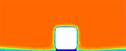
As known from the above analysis, the flow field around the sides could be effectively reduced through installing side windshields. On this basis, full windshields were installed at the connection section, and the computational method was also applied to compute flow field characteristics of both the high-speed train and connection sections, whose results were shown in Fig. 9-Fig. 11. It was shown that the flow field characteristics distributed symmetrically around the high-speed train, which was mainly caused due to its highly symmetrical structure. When the fluid was flowing backwards from the head, the structural heights contacted by fluid on both sides of the longitudinally symmetrical plane were consistent. Besides, as known from the flow field distribution characteristics of the entire train, maximum pressure was on the nose tip of the high-speed train head; and higher positive pressure area could be easily formed in this region due to severe deformation existing in this structure, and the bogie, wheels and other complex structural models emerged in the lower section of the train body. Such conclusion was also reflected in turbulence intensity distribution in Fig. 11.
Fig. 9Pressure distribution around the high-speed train

a) Pressure distribution of entire trains

b) Pressure distribution of the connection section
It was shown from Fig. 9(b) that after installing full windshields in the connection section of the train, the pressure distribution in the connection section was highly uniform, which was significantly improved compared with the result in Fig. 6. It was because windshields can prevent the flow of fluid effectively. As shown from Fig. 10(b), after installing full windshields in the connection section, the flow velocity of the fluid was gradually decreased from the outside to the inside, whose distribution was substantially consistent in various surfaces. The fluid was still flowed downwards along both sides, with the decreasingly flow velocity. Besides, as seen from the comparison of Fig. 11(b) and Fig. 8(b), after installing full windshields in the connection section, only a relatively large turbulence was formed in the roof region away from the connection section rather than at the corner of the step.
Fig. 10Flow velocity distribution of the fluid around the high-speed train

a) Flow velocity distribution of the fluid in entire trains
b) Flow velocity distribution of the fluid in the connection section
Fig. 11Turbulence intensity distribution around the high-speed train

a) Turbulence intensity distribution of entire trains

b) Turbulence velocity distribution of the fluid in the connection section
5. Computations of radiation noises in the connection section of the high-speed train
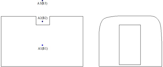
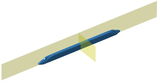
The structural vibration and externally radiation noises would be caused by the flow of fluid in the connection section, thus affecting the operating environment of the train. The above flow field results were imported into the acoustics software Virtual.Lab. Then, the acoustic boundary element model was also introduced into the software. Finally, the flow field results were mapped to the boundary element mesh in order to obtain all flow field features of the mesh, thereby conducting on the acoustic coupling computation and obtaining the acoustic radiation field around the connection section. Six observation points were arranged in the cross section of the connection section, as shown in Fig. 12. Among them, A1, A2, and A3 were at the distance of 3 m away from the longitudinally symmetrical plane of the train, and at the height of 1 m, 2 m and 3 m away from the ground, respectively. B1, B2 and B3 were at the distance of 7m away from the longitudinally symmetrical plane of the train, and at the height of 1 m, 2 m and 3 m away from the ground, respectively. The reason why the observation points were chosen to be 3 m and 7 m away from the longitudinally symmetrical plane of the train was that we wanted to compare and analyze the near-field and far-field radiation noises of the train in the connection section. The train was 2.5 m wide. Therefore, the purpose of choosing the observation point which was 3 m away from the longitudinally symmetrical plane of the train was to observe the near-field radiation noise. We did not choose the observation point which was 2 m away from the longitudinally symmetrical plane of the train because we found it difficult to arrange a microphone to measure the radiation noise in that position. We chose the observation point which was 7 m away from the longitudinally symmetrical plane of the train because wind tunnel test has limited width and we found it impossible to choose further observation points. Therefore, the final simulation and test chose 3 m and 7 m away from the longitudinally symmetrical plane of the train as the observation point.
Fig. 12Positions of measuring points of high-speed train
5.1. Side windshields
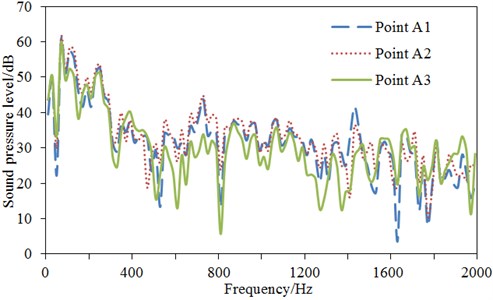
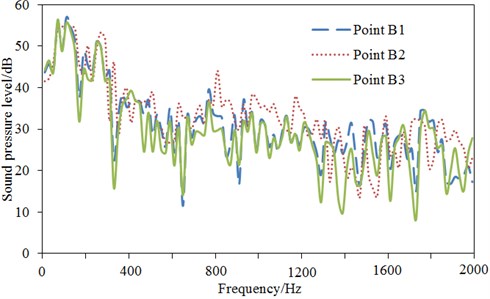
As shown from analysis of Section 4, the flow field distribution of the high-speed train was highly symmetrical. Therefore, only half models of the high-speed train were chosen as the research object during computing sound field of the high-speed train, which could reduce the computational time and improve the computational efficiency. The boundary element mesh was divided according to the geometric model of the high-speed train, whose results were shown as Fig. 13. Observation points were arranged in the cross-section of the connection section of the train and longitudinally symmetrical plane of the train, respectively, so as to observe the external radiation noise characteristics of the train, thus obtaining the boundary element model as shown in Fig. 14. Then, the computational flow field was imported into the software and coupled with the acoustic boundary element model, so as to compute the sound field of two observation planes. SPLs at the observation point in Fig. 12 were extracted to obtain the results shown in Fig. 15.
Fig. 13Boundary element meshes of the high-speed train
As shown in Fig. 15(a), SPL trends and values at points A1 and A2 were similar, while more valley values were appeared at point A3. Maximum SPLs at three points were around 100 Hz, and the maximum one was 62.1 dB. The minimum value 3.2 dB of observation point A1 was appeared near the frequency of 1650 Hz, with the great difference between the minimum and maximum values. Across the entire spectrum, four obvious peaks of 62.1 dB, 53.2 dB, 47.6 dB and 42.2 dB were at observation point A1, and their corresponding frequencies were 100 Hz, 246 Hz, 721 Hz and 1465 Hz, respectively. In addition, there were five obvious valleys of 22.1 dB, 12.1dB, 12.3 dB, 3.2 dB and 9.5 dB, respectively, with the corresponding frequency of 47.6 Hz, 574.2 Hz, 812.1 Hz, 1650 Hz and 1800 Hz, respectively. A2 showed similar trend to A1, and A3 presented a similar change to A1 and A2 within 400 Hz; but when the frequency was increased, A3 as a bandwidth noise, showed relative minimal fluctuations in the entire spectral range because aerodynamic noise played a major role in the high frequency. The average SPL of three observation points was computed, and the corresponding value was 31.8 dB, 33.2 dB and 30.1 dB, which indicated that the radiation noise of observation point A3 was the smallest. A3 was at a distance 3 m away from the ground, which was already at the top of the connection section, whose spectral characteristics of noises were slightly different from the other points.
Fig. 14Boundary element model of the high-speed train
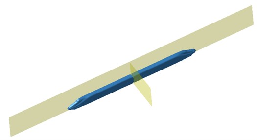
Fig. 15Comparisons of SPLs at observation points of the high-speed train
a) Comparisons of SPLs at observation points of 3 m
b) Comparisons of SPLs at observation points of 7 m
As shown from Fig. 15(b), sound pressure distributions of points B1 and B3 were similar, both presenting many peaks and valleys. Maximum SPLs at three observation points were still around 100 Hz, and the maximum one was 57.4 dB. The minimum SPL value 8.2 dB among three observation points was at point B3 near the frequency of 1750 Hz, with the great difference between the minimum and maximum values. Across the entire spectrum, many obvious peaks of 32.2 dB, 14.1 dB, 12.1 dB, 11.5 dB, 9.3 dB, 11.6 dB and 8.2 dB were at observation point B3, and their corresponding frequencies were 187 Hz, 372 Hz, 635 Hz, 1300 Hz, 1400 Hz, 1600 Hz and 1750 Hz, respectively. The average SPL of three observation points was computed, and the corresponding value was 31.2 dB, 33.1 dB and 29.2 dB. It could be seen that denser sound pressure valleys were distributed in the high frequency range over 1000 Hz. Moreover, as seen from the comparison of Fig. 15(a) and 15(b), SPL at the distance of 3 m was greater than that of 7 m, primarily because no obstacles were in the spreading space from 3 m to 7 m so that the sound was mainly attenuated through the dissipation of heat energy transited from air friction.
Fig. 16Sound pressure distribution contours at observation points of the high-speed train
a) 50 Hz
b) 100 Hz
c) 500 Hz
d) 1000 Hz
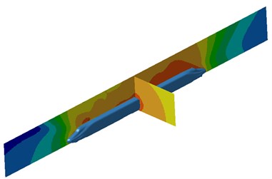
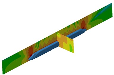
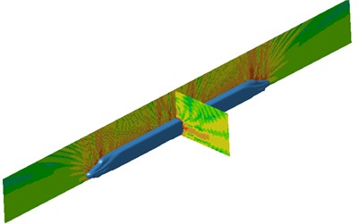
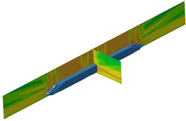
Sound pressure distribution contours at field points of 50 Hz, 100 Hz, 500 Hz and 1000 Hz were extracted, with the results shown in Fig. 16. It was shown that obviously great SPL was in the connection section at 50 Hz, and SPL distribution in the longitudinally symmetrical plane was greater in the tail of the train than the head. At 100 Hz, the sound pressure in cross-section of the connection section distributed in the region of 7 m, and a periodic attenuation of sound pressure distributed in the longitudinally symmetrical plane of the train, which was maximum in the head and tail of the train. It was because the longitudinal dimension of the high-speed train was much larger than the lateral dimension. As a result, the high-speed train can be seemed as a beam structure. The mode of a beam structure presented a periodicity, and then the radiation noise would present a periodicity. As a result, sound pressure distribution on the high-speed train had an obvious periodicity. SPLs of the head and tail were reduced and mainly distributed in the middle section at 500 Hz and 1000 Hz, and the sound had presented significant directivity and radiated externally from the surface of the train body with greater radiation distance. It was because there was a big pressure differential on the train head, serious structure change and eddies in the tail of the high-speed train. At two frequencies, a distinct directional sound pressure contour was appeared in the cross-section of the connection section, including observation points A2 and B2. Therefore, relatively large sound pressure in A2 and B2 was shown in the 500 Hz-1000 Hz, as shown from Fig. 15(a) and Fig. 15(b).
5.2. Full windshields
The aerodynamic noise of the high-speed in the above was only analyzed under installing side windshields in the connection section. Similar to the above analysis, the aerodynamic noise of the high-speed should also necessarily be computed under installing full windshields in the connection section. As a symmetrical structure, the half model of the high-speed train was therefore selected for the study, and the boundary element mesh of the high-speed train was shown in Fig. 17. Furthermore, observation points were arranged in the cross-section and longitudinally symmetrical plane of the train respectively, so as to observe the external radiation noise characteristics of the train, which obtained a boundary element model as shown in Fig. 18. Then, the computational results were imported into the software and coupled with acoustic boundary element model to compute sound fields of two observation planes. SPLs at observation points in Fig. 12 were extracted, whose results were shown in Fig. 19.
Fig. 17Boundary element meshes of the high-speed train
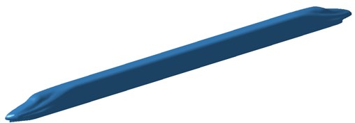
Fig. 18Boundary element model of the high-speed train
SPLs of observation points at the distance 3 m away from the longitudinally symmetrical plane of the high-speed train were shown in Fig. 19(a). It was shown that SPL trends of three observation points were basically same, especially at the frequency less than 1200 Hz. Maximum SPLs of three observation points were in near 50 Hz, and the largest one was 59.2 dB. The minimum SPL value 2.3 dB of observation point A3 was in near 2000 Hz, with the great difference between the minimum and maximum values. Only SPL curves of observation point A3 of three observation points presented many valley values which were 27.4 dB, 20.1 dB, 15.2 dB, 15.3 dB, 8.1 dB and 2.3 dB, and the corresponding frequency points were 200 Hz, 621 Hz, 901 Hz, 1123 Hz, 1506 Hz and 2000 Hz respectively. The average SPLs of three observation points were computed and the corresponding result was 29.6 dB, 30.0 dB and 28.4 dB, respectively. When the analyzed frequency was from 1200 Hz to 1400 Hz, SPLs of observation point A3 was significantly smaller than that of other two observation points. When the analyzed frequency was from 1400 Hz to 1600 Hz, SPLs of observation point A3 presented an obvious valley value. The SPL curve of observation point A3 was different from that of other two observation points because the distance of observation point A3 from the ground was greater than that of other two observation points and observation point A3 was relatively less affected by windshields.
Fig. 19Comparisons of SPLs at observation points of the high-speed train
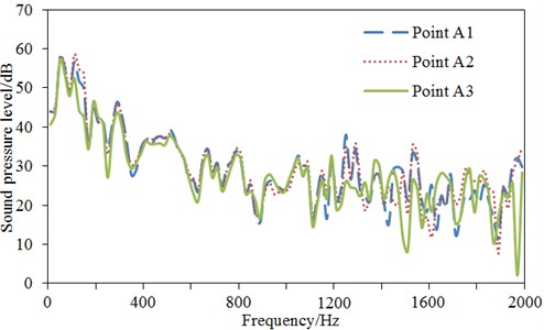
a) Comparisons of SPLs at observation points of 3 m
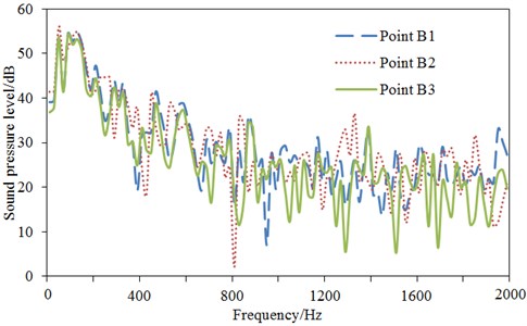
b) Comparisons of SPLs at observation points of 7 m
SPL comparisons at observation points of 7 m away from the longitudinally symmetrical plane of the high-speed train was shown in Fig. 19(b). It was shown that three observation points had presented obviously different SPL trends, and all of their maximum value 57.2 dB was shown in near 50 Hz. Minimum SPL value 2.4 dB of observation point B2 were in near 800 Hz, with the great difference between the minimum and maximum values. Similarly, more obvious valleys of 14.3 dB, 15.2 dB, 6.2 dB, 6.3 dB and 7.4 dB were at observation point B3, and their corresponding frequencies were 821 Hz, 1076 Hz, 1300 Hz, 1521 Hz and 1700 Hz, respectively. Average SPLs of three observation points were computed to obtain 28.5 dB, 28.6 dB and 26.0 dB. It could be noted that the average SPL of observation point B3 was relatively smaller mainly because three observation points were 7 m away from the longitudinally symmetrical plane of the train and observation point B3 was 3 m away from the ground, and relatively less affected by the aerodynamic noise of the train. Moreover, as seen from the comparison of Fig. 19(a) and Fig. 19(b), SPLs at the distance of 3 m from the symmetrical plane was numerically greater than that of 7 m. And relatively more peaks and valleys were shown in the SPL of 7 m.
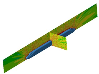
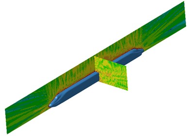
Sound pressure distribution contours at field points of 50 Hz, 100 Hz, 500 Hz and 1000 Hz were extracted, with the results shown in Fig. 20. It was shown that SPLs in the longitudinally symmetrical plane of the connection section at 50 Hz was greater than other frequency points, which was similar to the SPL curve in Fig. 19. Furthermore, the radiation noise in longitudinally symmetrical planes of the head and tail of the high-speed train was asymmetrical, with relatively greater value in the tail. At 100 Hz, a periodic change was also shown in SPLs of symmetrical plane of the high-speed train, which was consistent with the result in Fig. 16. At 500 Hz and 1000 Hz, a significant directivity was also in SPLs of the high-speed train, whose directivity distribution was denser than that of Fig. 16.
Fig. 20Sound pressure distribution contours at observation points of the high-speed train
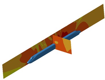
a) 50 Hz
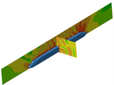
b) 100 Hz
c) 500 Hz
d) 1000 Hz
Fig. 21Comparisons of SPLs for three kinds of trains
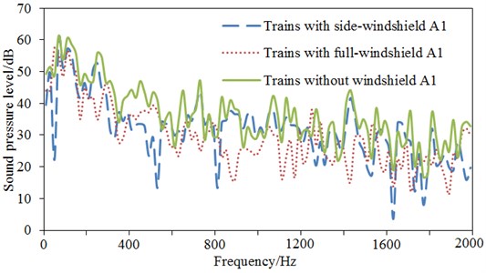
Side windshields and full windshields installed in the connection section were only studied longitudinally in the above, while lateral researches were ignored. A1 on the same horizontal plane was taken as the example for SPL comparisons, whose results were shown in Fig. 21. It could be seen that the SPL of trains without installing any windshields was basically higher than that of trains with windshields in the analyzed frequency, which indicated that windshields could efficiently reduce the radiation noise of the train in the connection section. The average SPLs of three kinds of trains were computed respectively to obtain 31.8 dB, 29.6 dB and 36.4 dB. The average SPL of trains without installing windshields was significantly greater than that of other two structures. In addition, it was shown that after installing full windshields, SPLs were significantly reduced at most frequency points when they were compared with the side windshields. At 1400 Hz, SPLs of side windshield were 38.9 dB while SPLs of full windshield were 15.3 dB, with the difference of 23.6 dB, indicating very apparent noise reduction effect. Moreover, SPL curves were relatively stable after installing full windshields. Therefore, the application of full windshields was very meaningful for the reduction of radiation noises in the connection section of the train and improvement of operating environment.
6. Experimental verification
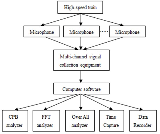
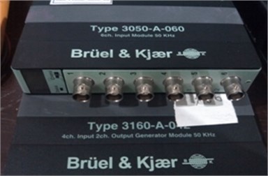
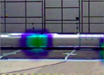
The computational process of aerodynamic noises for the high-speed train was relatively complex, and only using numerical simulation was difficult to show the reliability of the studied result. Therefore, experiments were necessarily required to verify the above studies. Three sensors were arranged at 3 m and 7 m away from the connection section of the head and tail of the train, respectively, according to Fig. 12, so as to test the external radiation noise in the connection section. Due to multiple noise sources, the characteristics of each noise source cannot be completely distinguished by the sensor. For such purpose, the sound source identification equipment was also applied in the test to locate and measure several major noise source positions. The entire process of the test was shown in Fig. 22. The multi-channel data acquisition device was employed in the test to collect test data, as shown in Fig. 23(a). The signal of sensors and sound source identification equipment were input into the computer, and then PULSE software was used to conduct post-processing for the test signal, thus obtaining the sound source distribution contour as Fig. 23(b). As can be seen from the figure, an obvious noise source was found in the connection section mainly because there was a structural change in the connection section. The flow state of flow field would be changed, which thus led to the change of sound field.
Fig. 22Noise test process of the connection section
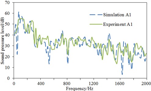
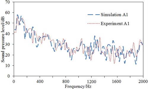
The tested sound pressure of the measurement points was compared with the above numerical result by taking A1 as the example, whose results were shown in Fig. 24. The comparison of experimental and numerical results after installing side windshields was shown in Fig. 24(a), presenting very similar trends between them. Compared with numerical simulation, not many valleys were in the experimental result. The comparison of experimental and numerical results of full windshields was also shown in Fig. 24(b), presenting a good agreement between them. As can be seen from the above analysis, the applied numerical simulation method and model herein were reliable, and the analyzed result and obtained conclusions were effective.
Fig. 23Equipment and result of noise test
a) Data acquisition device
b) Noise source distribution
Fig. 24Comparisons of experimental and simulation SPLs in two kinds of windshields
a) Comparisons of experimental and simulation SPLs in side windshields
b) Comparisons of experimental and simulation SPLs in full windshields
7. Conclusions
1) The flow field distribution characteristics of side windshields and full windshields installed in the connection section of a high-speed train were numerically computed. As shown from the result, the maximum pressure was at the nose tip of the high-speed train; and the greatest flow velocity of fluid was centered in the middle section of the body, while the flow velocity at both ends of the body was relatively small. After installing a side windshield, the fluid pressure of the side was significantly lower than the upper and lower surfaces, and the pressure and turbulence intensity were greater at the corner of the connection section steps. The fluid flowed to the steps from the roof of the train, and then spread gradually down along the side, with the decreasing flow rate. Therefore, the airflow was effectively prohibited from flowing into the train through installing side windshields. However, after further installing full windshields, the pressure, flow velocity and turbulence intensity in the connection section of the high-speed train were further improved.
2) Then, the boundary element method was applied to compute the radiation noises of two kinds of windshields installed in the connection section of the high-speed train. As shown from the result, broadband radiation noise was in the upper connection section, the maximum sound pressure level (SPL) value was between 50 Hz-100 Hz and some directivity of sound pressure was shown in the high-frequency range. A certain periodicity of sound pressure distribution was presented in the longitudinal symmetrical plane of the high-speed train. At the same observation point, the sound pressure level of full windshield was slightly reduced at most frequency points, and the maximum reduction value was 23.6 dB.
3) Finally, the wind tunnel test was conducted on the high-speed train, and the connection section of the high-speed train was the obvious noise source, thus indicating that the research in the paper was very meaningful. Besides, from SPL comparisons of the observation point, experiments and simulations were consistent with each other whether side windshields or full windshields were installed in the connection section. As a result, the reliability of the numerical computational model and the effectiveness of the results and analysis were verified.
References
-
Shen Z. Y. Dynamic environment of high-speed train and its distinguished technology. Journal of the China Railway Society, Vol. 28, Issue 4, 2006, p. 1-5.
-
King W. F., Bechert D. Aerodynamic noise generated by high speed trains. Noise Control Engineering, Vol. 13, 1979, p. 13-23.
-
Nagakura K. Localization of aerodynamic noise sources of Shinkansen trains. Journal of Sound and Vibration, Vol. 293, 2006, p. 547-556.
-
Nagakura K. The Methods of Analyzing Sinkansen Noise Railway. Technical Research Institute, Quarterly Reports, Vol. 37, 1996, p. 210-215.
-
Zhang S. G. Noise mechanism, sound source localization and noise control of 350 km/h high-speed train. China Railway Science, Vol. 30, Issue 1, 2009, p. 86-90.
-
Frid A. Skirts and barriers for reduction of wayside noise from railway vehicles-an experimental investigation with application to the BR185 locomotive. Journal of Sound and Vibration, Vol. 267, Issue 3, 2003, p. 709-719.
-
Kitagawa T., Nagakura K. Aerodynamic noise generated by Shinkansen cars. Journal of Sound and Vibration, Vol. 231, Issue 5, 2000, p. 913-924.
-
Ikeda M., Morikawa T., Manade K. Development of low aerodynamic noise pantograph for high speed train. International Congress on Noise Control Engineering, Vol. 1, 1994, p. 169-178.
-
Ikeda M., Suzuki M., Yoshida K. Study on optimization of pan-head shape possessing low noise and stable aerodynamic characteristics. Quarterly Report of Railway Technical Research Institute, Vol. 47, Issue 2, 2006, p. 72-77.
-
Iwamoto K., Higashi A. Some consideration toward reducing aerodynamic noise pantograph. Japanese Railway Engineering, Vol. 122, Issue 2, 1993, p. 1-4.
-
Sassa T., Sato T., Yatsui S. Numerical analysis of aerodynamic noise radiation from a high-speed train surface. Journal of Sound and Vibration, Vol. 247, Issue 3, 2001, p. 407-416.
-
Xiao Y. G., Tian H. Q., Zhang H. Prediction of interior aerodynamic noise of high-speed train cab. Journal of Traffic and Transportation Engineering, Vol. 8, Issue 3, 2008, p. 10-14.
-
Shi X. G. Turbulence. Tianjing University Publishing House, Beijing, 1977, p. 125-128.
-
Felten F., Fautrelle Y., Du Terrail Y., et al. Numerical modeling of electrognetically-riven turbulent flows using LES methods. Applied Mathematical Modelling, Vol. 28, Issue 1, 2004, p. 15-27.
-
Hong S. H., Dong N. G., Wu Y. N. A study on aerodynamic noise simulation for a SUV rear view mirror. Vehicle and Power Technology, Vol. 4, 2007, p. 39-42.
