A hybrid fault diagnosis method for mechanic-electronic-hydraulic control system based on simulated knowledge from virtual prototyping

1. Introduction

With the rapid development of modern industrial technology, mechanic-electronic-hydraulic control systems (MEHCS) have been being used more and more widely. While they are liberating human with their high efficiency, convenience and accuracy, on the other hand, are bothering human when faults happen to them. Therefore, it’s very urgent that MEHCS be monitored and diagnosed under real-time working condition. For simple control systems, there may be relatively more colorful fault diagnosis methods available. But as the control systems become more and more complicated and larger, effective diagnosis approaches are being restricted for practical application, especially on system-level.

Generally speaking, fault diagnosis methods for control system could be classified into three categories: mathematical model-based method, signal processing-based method and knowledge-based method. Their detailed literature review and comparison will be presented in the next section. To sum up, for the fault diagnosis of large-scale and complicated control system, knowledge-based method is more appropriate than the other two. However, knowledge-based method has its own inherent disadvantage. Because the actual systems are usually working under normal condition, data under faulty condition is lacking seriously [1]. What’s more, for large-scale and complicated MEHCS, the amount of the same systems in service is very small. Fault database is hard to build and complete in the entire industrial field. These two reasons lead to the lack of historical fault data, which is the main source of objective knowledge for fault diagnosis. On the other hand, experts’ experience is also hard to accumulate because of the similar reasons.

Recent years, with the rapid development of computer technique, simulation-based methodologies have been used in almost every domain of scientific research and social practice. This is mainly because of the good flexibility, low cost and high efficiency of simulation technique. As an important branch of simulation technique, virtual prototyping has been developing rapidly since 1980s. Virtual prototyping is a digital model built on software platform which can imitate the original system’s functions that people are interested in. This paper is trying to apply virtual prototyping to fault diagnosis of MEHCS. Diagnosis knowledge derived from simulation data is supposed to make up the lack of historical fault data and experts’ experience.

As stated above, this paper proposes a hybrid fault diagnosis method for MEHCS based on simulated knowledge from virtual prototyping, which is trying to deal with the lack of historical fault data for the knowledge-based fault diagnosis methods, especially for large-scale and complicated cases. The rest part of this paper is arranged as follows. In Section 2, current methods developed for the fault diagnosis of control system will be reviewed and summarized. In Section 3, the hybrid diagnosis method based on simulated knowledge from virtual prototyping will be proposed and illustrated in detail. In Section 4, a case study of vessel steering system will be presented to verify the proposed methodology. Conclusion and discussion will be finally made in Section 5.

2. Literature review

Generally speaking, fault diagnosis is supposed to perform three tasks: fault detection, fault isolation and fault identification (FDII) [2]. Fault detection is to make a decision that whether system has a fault. Fault isolation is to determine the location of the fault. Fault identification is to estimate the severity or nature of the fault. Fault detection and isolation (FDI) can fulfill the demand of ordinary fault diagnosis. Fault identification, however, is important for fault recovery and health monitoring but is not concerned in this paper. Fault diagnosis methods for control system, according to their basic principle, could be classified into three categories: mathematical model-based methods signal processing-based methods and knowledge-based methods.

Mathematical model-based methods analyze the residual signal between actual system and its mathematical model. Three approaches are usually employed to generate residuals. They are observer-based (or filter-based or state estimation-based) approach [3], parity space approach [4] and parameter estimation approach [5]. The foundation of mathematical model-based method is to get the accurate mathematical model of actual system. For small-scale and simple systems, this work could be achieved easily using traditional dynamic modeling approach based on physical mathematics. For large-scale and complicated cases, however, this work would be extremely time-consuming and effort-exhausting. Because the details of components and their combination are usually complex and uncertain, accurate mathematical model is hard to obtain.

Signal processing-based methods analyze the system measured signals from sensors and could be divided into two approaches. The first approach is time domain threshold test or trend analysis which extracts trend features in time domain of signals [6]. The second approach is frequency (such as discrete Fourier transform, DFT) or mixed time-frequency domain (such as discrete wavelet transform, DWT) analysis which extracts features in frequency or mixed time-frequency domain. Signal processing techniques are mainly applied to the fault diagnosis of machinery components such as bearing and gearbox [7, 8]. They usually do not consider the interrelationship between the measured signals, which results in increasing the risk of false alarm. And sometimes the diagnosis result couldn’t correspond to the real system well and has confused meaning. What’s more, some approaches can only be capable of the diagnosis of specific fault of specific component.

Knowledge-based methods rely on the historical data and experts’ experience of system. The former approaches are to learn the system model from the historical input-output data. The learned data-driven model can then be used to generate residual signal. Such methods are also known as computational intelligence-based methods or artificial intelligence-based methods, including artificial neural networks [9] and fuzzy logic [10]. Alternatively, historical data can also be used to build knowledge database for fault diagnosis based on pattern recognition, which will be utilized in this paper. The later approaches use the experts’ experience encoded as a series of if-then rules, including expert system [11] and fault tree [12]. The main drawback of knowledge-based methods is relying too much on the historical data or experts’ experience, which leads to a strong subjectivity. Detailed contrast and summary of the three categories of fault diagnosis method are listed in Table 1.

As stated above, for the diagnosis of large-scale and complicated MEHCS, mathematical model-based methods are difficult to apply because the obtainment of accurate mathematical model is too hard. On the other hand, signal processing-based methods can only be capable of the diagnosis of specific fault of specific component, so they are not capable of fault diagnosis on system-level. As a result, knowledge-based methods may be the most appropriate one. However, “Even a clever woman cannot cook a meal without rice”. The knowledge-based methods rely on the historical data or experts’ experience of system. But the historical data, especially fault data and experts’ experience is hard to accumulate for large-scale and complicated MEHCS. This is the main bottleneck that restricts these methods for being applied in practice.

3. Hybrid diagnosis method based on simulated knowledge from virtual prototyping

As stated in the above section, mathematical model-based, signal processing-based and knowledge-based methods all have their individual inherent disadvantages. But for the fault diagnosis of large-scale and complicated MEHCS, knowledge- based methods are more appropriate. In order to overcome the lack of historical fault data, a hybrid fault diagnosis method based on simulated knowledge from virtual prototyping is proposed in this paper. This method could be divided into four stages as illustrated in Fig. 1.

The first stage is to establish the virtual prototyping. As stated above, it’s too hard to get the system model using traditional dynamic modeling approach based on physical mathematics. With the rapid development of simulation techniques, many dynamic modeling platforms have been developed. With these platforms, large-scale and complicated systems could be modeled according to the basic constitutions and compositions of them. The established model is called “virtual prototyping”, which can describe the basic principle and function of the actual system. It could also reveal the primary energy transfer forms of the system, such as force, electric and hydraulic pressure.

However, before being used for intended need, virtual prototyping must be verified and validated to ensure its credibility. Verification and validation (V&V) is thus the significant foundation of the proposed method, which shall be paid enough attention to. It should be pointed out that V&V should be conducted throughout the whole lifetime of modeling and simulation rather than being taken as a terminal work.

The second stage is data obtainment. Simulation data is the source of simulation knowledge. Fault injection and fault simulation are inevitable for data obtainment. Fault injection is to imitate the fault in actual system by changing parameters, adding/reducing components and/or other means in the virtual prototyping. Fault simulation is to simulate the fault model by assign initial parameters, sample interval and simulation time, etc. For every simulation, simulation data of the measure points that we are interested in could be collected and thus the effect of the injected fault could be analyzed.

Fig. 1The four stages of the proposed methodology

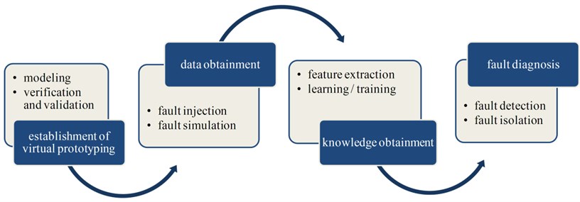
Simulation data should be as comprehensive as possible for getting comprehensive knowledge, which asks the fault simulations covering working conditions as many as possible. Working condition includes a series of random variables. Therefore, the probabilistic distributions of the most pivotal variables should be appointed. On this basis, Monte Carlo method is used to sample these variables. One set of sample values is used in an individual fault simulation. By performing enough fault simulations, fault database could be built and improved gradually.

The third stage is knowledge obtainment. According to the fault simulation results, all the fault modes could be classified into several fault types. For a specific fault type, fault features could be extracted. Feature extraction can reduce the data amount for storing and increase the efficiency of training and diagnosis. On this basis, three pattern recognition methods are used to train the extracted fault features, including probabilistic neural network (PNN), naive Bayes (NB) and $k$-nearest neighbor (kNN). As a result, knowledge libraries for fault diagnosis are built. Every fault type has its individual knowledge database. This arrangement is also supposed to increase the accuracy and efficiency of fault diagnosis.

The fourth stage is fault diagnosis. The proposed method is trying to realize real-time condition monitoring and fault diagnosis. Firstly, decision is made about whether the system has a fault and what type the fault is, using threshold test according to the input-output characteristic of the system. This procedure essentially realizes fault detection. On this basis, fault mode is recognized according to the measured data by using the fault diagnosis knowledge database corresponding to the fault type. An ensemble classifier constructed by the above three pattern recognition methods is employed in this process. This procedure essentially realizes fault isolation.

In the proposed methodology, fault diagnosis is realized base on the simulated knowledge from virtual prototyping. Virtual prototyping could be treated as a special type of mathematical model. Thus the proposed method is essentially a hybrid fault diagnosis method based on mathematical model and knowledge. The lack of historical fault data in knowledge-based methods is overcame by the employment of virtual prototyping. In addition, virtual prototyping could be easily obtained by the using of modeling software. In summary, the proposed method is supposed to take the advantages of model- based and knowledge-based methods, and avoid their disadvantages.

4. Case study

The object of study is a vessel steering system, which is a typical double closed-loop mechanic- electronic- hydraulic servo control system used to control the angle of vessel rudder. The system consists of rudder-operating unit, pump-control unit, control circuit, rudder cylinder and rudder angel feedback unit, etc. Rudder angle is controlled by servo route to follow the command given by operator or computer. The basic principle of this system is illustrated as Fig. 2(a) [13]. Order angle is given by operating device and is then demodulated and subtracted by the actual rudder angle. The subtracted signal was then amplified, sampled and subtracted by the feedback from displacement sensor for flushing plate. Thus the inner closed-loop is essentially used to control the displacement of flushing plate, which controls the flow rate and direction of pump directly. In Fig. 2(a), 1#-7# are measure points used for the verification and validation of the virtual prototyping. For every point, appropriate sensor or sensing wire are installed and connected to data collector. Thus the actual signal could be measured and collected to be contrasted with the simulated signal.

Fig. 2Control principle and virtual prototyping of steering system

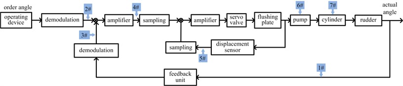
a) Control principle of steering system

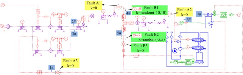
b) Virtual prototyping of steering system and the fault injection details

4.1. Establishment and V&V of virtual prototyping

AMESim was chosen as the modeling platform. Steering system was divided into several functional modules based on its working principle and constitution. Appropriate components in corresponding libraries were chosen to build every functional module. Lastly, interfaces among the modules were designed. The established virtual prototyping of steering system is illustrated as Fig. 2(b). In Fig. 2(b), 1#-7# are measure points used for the verification and validation of the virtual prototyping, which corresponds to the measure points in Fig. 2(a) respectively. For every point, virtual measure points could be set in AMESim and simulated signal could be saved to be contrasted with the simulated signal. Diagrams of fault A1, A2, A3 and B1, B2 and B3 illustrate the fault injection details in AMESim. For every fault model, the dotted circle is replaced by the module in the relevant diagram or the parameter in the dotted circle is modified as in the diagram.

Before being used for intended need, virtual prototyping must be verified and validated to ensure its credibility and accuracy. Verification cares about: “Did I build the model right?” Validation, however, cares about: “Did I build the right model?”. Verification and validation is the basis of application of modeling and simulation and is thus very significant.

Generally speaking, V&V is to prove and guarantee that the established model is similar enough to the real system for intended use. Detailed introduction and explanation about V&V could be found in [14], which is not focused in this paper. However, as the key procedure of V&V, “results validation” will be presented in detail. Result validation means validating the results from the real system and virtual prototyping under the same input. Thus it is inevitably that make a contrast between the measured signal and simulated signal. In order to make such contrast quantitatively, appropriate similarity measures should be well designed. Similarity measures are very important as it is the vital link from real system to virtual prototyping. Suppose that $x_t$ and $y_t$ are the observation series of real system signal $X$ and virtual prototyping signal $Y$ respectively. Thus the error between them is:

1

$e_t=\mathrm{}{x}_t-y_t,t=1,\mathrm{}2,\dots ,N,$

where$N$ is the length of the series. In this paper, correlation coefficient ${\rho }_{X,Y}$ is used to describe the trend similarity between two data series and the relative (to the theoretical maximum amplitude of observation series) value of Root-Mean-Square (RMS) of error ${\lambda }_{X,Y}$ is taken as the amplitude similarity measure:

2

${\rho }_{X,Y}=\frac{\sum _{t=1}^N\left(x_t-\overline{x}\right)\left(y_t-\overline{y}\right)}{\sqrt{\sum _{t=1}^N{\left(x_t-\overline{x}\right)}^2\sum _{t=1}^N{\left(y_t-\overline{y}\right)}^2}},$

3

${\lambda }_{X,Y}=1-\frac{{RMS}_e}{A_{\mathrm{m}\mathrm{a}\mathrm{x}}},$

where $\stackrel{-}{x}$ and $\stackrel{-}{y}$ are the mean of $x_t$ and $y_t$ respectively, ${\mathrm{R}\mathrm{M}\mathrm{S}}_{\mathrm{e}}$ is the RMS of$e_t\text{,}$$A_{\mathrm{m}\mathrm{a}\mathrm{x}}$ is theoretical maximum amplitude of observation series. Eqs. (2), (3) could represent the real system signal and virtual prototyping signal in two critical aspects: trend and amplitude. ${\text{0}<\rho }_{X,Y}<\text{1}$ and $\text{0}<{\lambda }_{X,Y}<\text{1}$. The bigger ${\rho }_{X,Y}$ is, the more similar $X$ and $Y$ are in trend aspect. The bigger ${\lambda }_{X,Y}$ is, the more similar $X$ and $Y$ are in amplitude aspect. Based on the above two similarity measures, a comprehensive similarity measure could be designed based on weight as:

4

$S_{X,Y}=\alpha {\lambda }_{X,Y}+\beta {\rho }_{X,Y},$

where $\text{0}\le \alpha ,\beta \le \text{1,}$$\alpha +\beta =\text{1}$ are the weights of amplitude similarity measure and trend similarity measure. Different weights could reflect different application characteristic and the subjectivity of accreditation.

In order to validate the results of virtual prototyping, a series of validation experiment was designed and implemented. Parts of the actual system and experiment plant and sensors are illustrated in Fig. 3. In one of the experiments, square wave with amplitude of 24° was taken as the governing rudder input, as illustrated in Fig. 4(a). Virtual prototyping was simulated under the input and the simulated signals of seven measure points were saved. Real system run under the input and measured signals of seven measure points were collected using data collector. The distribution of measure points is illustrated in Fig. 2(a) and (b) as 1#-7#.

The contrast between simulated value and measured value of 1#, 4#, 5# and 7# measure points are illustrated in Fig. 4(b)-4(e). It could be judged visually that they are highly similar. In order to make quantitative judgment, similarity measures designed in the above section were calculated as shown in Table 2, where$\alpha =\beta =\text{0.5}$. If the threshold regulated in V&V plan is 0.95, the results could pass the validation. However, if the threshold is 0.97, the 4# measure point doesn’t fulfill the requirement. This would lead to the modification of virtual prototyping and repeating V&V activity. Different intended use may lead to different requirement of time series similarity. The validation results show that the virtual prototyping has a high similarity to the actual steering system and is credible/ acceptable.

Fig. 3Parts of the actual steering system and experiment plant: 1 – pump control subsystem; 2 – hydraulic pressure sensor; 3 – cylinder; 4 – loading plant; 5 – displacement sensor of cylinder rod; 6 – data collector; 7 – industrial computer

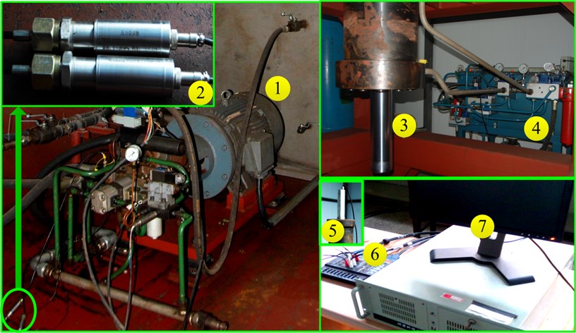
Table 2Similarity measures

Measure point	Theoretical amplitude	${\rho }_{X,Y}$	${\lambda }_{X,Y}$	$S_{X,Y}$
1#	25 (°)	0.99	0.96	0.98
2#	10 (V)	0.98	0.97	0.98
3#	10 (V)	0.99	0.99	0.99
4#	10 (V)	0.96	0.95	0.96
5#	10 (V)	0.97	0.96	0.97
6#	10 (MPa)	0.99	0.96	0.98
7#	10 (MPa)	0.99	0.95	0.97

4.2. Data acquisition

Fault injection is the core and basis of fault simulation which could be implemented in two ways. (1) Modifying the structure of virtual prototyping. Virtual prototyping could be transformed from nominal condition to faulty condition by adding or reducing some relevant components on the software platform. (2) Modifying the parameters of relevant components. Some parameters could control the generation of fault and thus could be modified to inject faults into virtual prototyping.

All typical fault modes are injected and simulated using some specific fault severity. According to the simulation results, fault modes could be classified into several basic fault types. In this study, there are mainly three fault types: stuck rudder (type A), steady state error (type B) and instantaneous state error (type C).

Stuck rudder means rudder angle stays as origin regardless of the change of order input. Except actuator fault, there are mainly three fault modes that could lead to stuck rudder. They are the output of outer amplifier is zero (Fault A1), the output of inner amplifier is zero (Fault A2) and the feedback of rudder angle is zero (Fault A3). The fault injection methods of these three fault modes are illustrated as yellow blocks in Fig. 2(b).

Fig. 4Contrast of simulated and measured signal

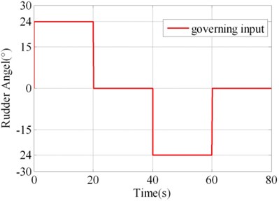
a) Governing input

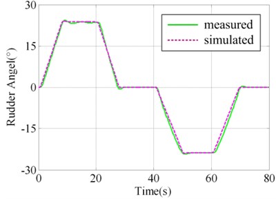
b) Measure point 1#

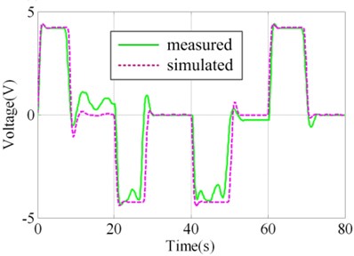
c) Measure point 4#

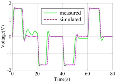
d) Measure point 5#

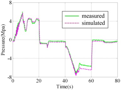
e) Measure point 7#

Steady state error means although the rudder changes according to the order, there is an offset between the steady rudder angle and ideal angle or the actual angle waves apparently around the order angle at steady state. There are also mainly three fault modes that can lead to steady state error. They are the outer amplifier has an offset (Fault B1), the feedback of flushing plate has an offset (Fault B2), and feedback of flushing plate is zero (Fault B3). The fault injection methods of these three fault modes are illustrated as green blocks in Fig. 2(b).

Instantaneous state error means although the rudder changes according to the order, there is an offset between the instantaneous rudder angle and ideal angle. In other words, the changing rate of rudder angle is different from normal condition. There are mainly three fault modes that can lead to instantaneous state error. They are: the outer amplifier has a gain (Fault C1), the feedback of flushing plate has a gain (Fault C2), and output of inner amplifier has a gain (Fault C3).

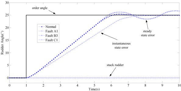
Simulation results of typical fault modes of the three fault types are illustrated in Fig. 5. Fault A1, B3 and C1 were simulated. The fault injection methods of these three fault modes are illustrated in Fig. 2(b). In the simulation, step order of 0° to 25° at 1 s is taken as the governing input angle as illustrated in Fig. 5 with the bold line. Normal and the above three faulty virtual prototyping models of steering system were simulated and the simulation results of actual angle are illustrated in Fig. 5. It could be inferred that fault type A is the riskiest type that may lead to the out of control of vessel rudder. Fault type B could also lead to the potential risk in critical condition. Comparatively speaking, fault type C is not so dangerous though it could decrease the efficiency of control. Therefore, type A and B are stressed in this paper.

Fig. 5Contrast of simulation result of three typical faults and normal state

Monte Carlo method is then employed in the fault simulation to get comprehensive fault data. Suppose that the initial rudder angle and order rudder angle are both random variables with a uniform distribution in [–25, 25]. The severities of fault B1 and B2 are uniform distributions respectively in [–5, 5] and [–10, 10]. The sample interval is 0.1 s. In every simulation trial, one set of random variables are sampled and numbers of simulation trials are implemented.

4.3. Knowledge obtainment

4.3.1. Feature extraction

Fault simulation data shall not be all used as knowledge for storing. This is because some fault data are not useful for fault diagnosis and, to the opposite, are negative sometimes. Thus it is necessary to extract the fault features that are useful for fault diagnosis.

Fault type A is both an instantaneous and steady fault type. To diagnose as early as possible, extracting instantaneous fault features is a more ideal choice. According to the analysis of instantaneous characteristics of steering system, the measured signals ought to change significantly at 0.5 s after order was given. Therefore, data points at 0.5 s of every measured signal are extracted as fault features and the rest of data points are given up. Another advantage of feature extraction could thus be seen that it can reduce the single simulation time to as short as 0.5 s. This is very favorable for increasing the efficiency of Monte Carlo simulation. For fault type A, the feature for fault detection is the difference between the current rudder angle and the initial rudder angle ($D_i$). The features for fault isolation are measure points MP3#, MP4, and MP5#. Fault features of 100 Monte Carlo simulations are illustrated in Fig. 6. Threshold for fault detection of type A could be determined according to the difference of $D_i$ between normal and faulty condition.

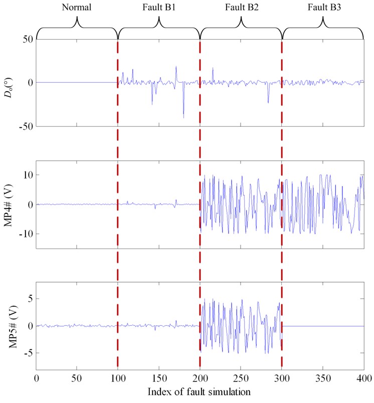
For fault type B, about 15 s will be cost for the rudder angle changing from –25° to 25° or for the contrast course. Thus, theoretically, steering system ought to be in steady state at 20 s after order was given. As a result, for fault type B, data points at 20 s of every measured signal are extracted as fault features. The feature for fault detection is the difference between the current rudder angle and the order rudder angle ($D_o$). The features for fault isolation are $D_o$, measure points MP4, and MP5#. Fault features of 100 Monte Carlo simulations are illustrated in Fig. 7. Threshold for fault detection of type B could be determined according to the difference of $D_o$ between normal and faulty condition.

Table 3Fault features extraction of fault type A and B

Fault types	Features
	Time point	Fault detection	Fault isolation
Type A	0.5 s	Current angle-initial angle ($D_i$)	MP3#	MP4#	MP5#
Type B	20 s	Current angle-order angle ($D_o$)	$D_o$	MP4#	MP5#

Fig. 6Fault feature of different fault modes of fault type A (from left to right: Normal, A1, A2 and A3)

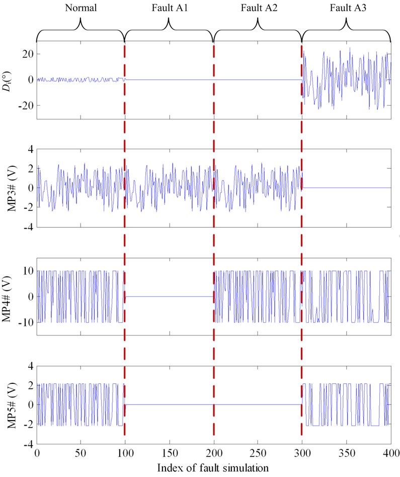
Fig. 7Fault feature of different fault modes of fault type B (from left to right: Normal, B1, B2 and B3)

4.3.2. Training

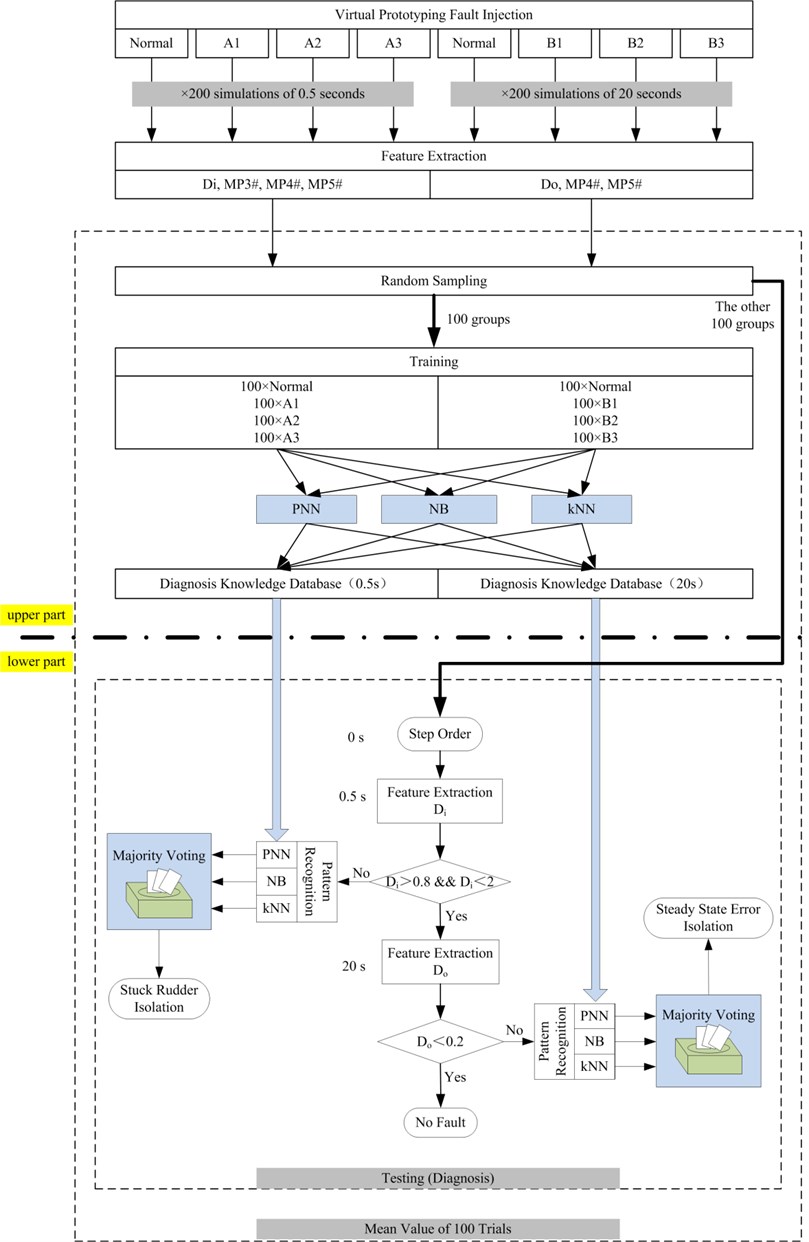
Take fault A for example. For three different fault modes under type A, three pattern recognition methods- probabilistic neural network (PNN) [15], naive Bayes (NB) [16] and $k$-nearest neighbor (kNN) [17] are respectively used for training. In order to get an ideal diagnosis result, enough amounts of training samples shall be ensured. However, as the amount becomes bigger, the time for training becomes longer and the data amount for storing becomes bigger at the same time. In this study, every fault mode has 100 samples. The procedure of fault simulation, feature extraction and training could be seen in the upper part of Fig. 8.

4.3.3. Ensemble classifier

The ensemble classifier employed in this paper is based on the principle of majority voting [18]. Majority voting is perhaps the simplest approach for combining classifiers and is commonly used [19]. It could be proven that if the accuracy is almost similar across the involved methods, majority voting has a better performance than any other more complicated combining rules [20].

4.4. Fault diagnosis result

Fault diagnosis strategy in this paper could be divided into two procedures, as is illustrated in the lower part of Fig. 8. Firstly, according to the features of fault detection at 0.5 s after order was given, decision could be made about whether a fault of type A happens based on threshold test. If the conclusion is “yes”, then knowledge database of type A will be utilized. Fault isolation could thus be conducted using an ensemble classifier constructed by PNN, NB and kNN. If the conclusion is “no”, decision could be made about whether a fault of type B happens at time point of 20 s. If the conclusion is “yes”, then knowledge database of type B will be utilized to isolate the fault. If the conclusion is “no”, the decision could be made that there is no fault right now.

Because of the lack of fault data of actual system, simulation data is used for validation. Take fault type A for example. There are totally 200 normal, A1, A2 and A3 samples respectively. In every validation experiment, 100 of them will be sampled randomly for training and the other 100 samples are used for testing. The testing result will be treated as the diagnosis result. 100 validation experiments will be conducted and the mean value will be investigated.

4.4.1. Fault type A

For fault detection of fault type A, the upper and lower limit of the threshold test is respectively 0.8 and 2. Thus the detection process could be expressed as:

5

$0.8\le D_i\le 2?\mathrm{}\mathrm{}\left\{\begin{array}{l}\text{Yes}\text{→}\text{no fault type A,}\\ \text{No}\text{→}\text{fault type A.}\end{array}\right.$

The average diagnosis results of 100 trials are listed in Table 4. In the 100 normal samples, 99.16 % are classified into “normal”. Thus the false alarm rate is 0.84 %. In the 300 fault samples, 98.99 % are classified into “fault”. Thus the missing alarm rate is 1.01 %. In the detected fault samples, the fault isolation accuracy of the three fault modes is respectively 100 %, 96.91 % and 94.83 % using PNN; 100 %, 97.75 % and 95.37 % using NB; 100 %, 95.78 % and 94.41 % using kNN. At last, ensemble classifier is employed. The corresponding isolation accuracy is 100 %, 96.80 % and 94.90 %.

Ideally, the ensemble classifier should perform better than any individual method. But the result may be somehow disappointing. However, the following paragraphs will analysis the results more deeply to suggest the advantages of ensemble classifier.

Table 4Fault diagnosis results of fault type A

Fault modes	Diagnosis result
	Detection accuracy	Isolation accuracy
Normal	99.16 %	PNN	NB	kNN	Ensemble classifier
Fault A1	98.99 %	100.00 %	100.00 %	100.00 %	100.00 %
Fault A2		96.91 %	97.75 %	95.78 %	96.80 %
Fault A3		94.83 %	95.37 %	94.41 %	94.90 %

4.4.2. Fault type B

For fault detection of fault type B, the upper limit of the threshold test is 0.2. Thus the detection process could be expressed as:

6

$D_o\le 0.2?\mathrm{}\mathrm{}\left\{\begin{array}{l}\text{Yes}\text{→}\text{no fault type B,}\\ \text{No}\text{→}\text{fault type}\text{B}\text{.}\end{array}\right.$

Fig. 8Flow path of the case study

The average diagnosis results of 100 trials are listed in Table 5. In the 100 normal samples, 99.16 % are classified into “normal”. Thus the false alarm rate is 0.84 %. In the 300 fault samples, 94.48 % are classified into “fault”. Thus the missing alarm rate is 5.52 %. In the detected fault samples, the fault isolation accuracy of the three fault modes is respectively 92.89 %, 84.55 % and 89.85 % using PNN; 87.86 %, 88.46 % and 87.41 % using NB; 92.88 %, 91.83 % and 95.58 % using kNN. At last, ensemble classifier is employed. The corresponding isolation accuracy is 92.91 %, 91.76 % and 94.88 %. These results are still not so “ideal” because they are not the best of all the three individual methods or better than any of them.

Table 5Fault diagnosis results of fault type B

Fault modes	Diagnosis result
	Detection accuracy	Isolation accuracy
Normal	100 %	PNN	NB	kNN	Ensemble classifier
Fault B1	96.97 %	92.89 %	87.86 %	92.88 %	92.91 %
Fault B2		84.55 %	88.46 %	91.83 %	91.76 %
Fault B3		89.85 %	87.41 %	95.58 %	94.88 %

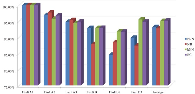
In order to show the advantages of ensemble classifier based on majority voting, a contrast analysis of the three individual pattern recognition methods and the ensemble classifier is presented. The average fault isolation results of using these four methods for all the fault modes are illustrated in Fig. 9. Average isolation accuracies are respectively 93.17 %, 92.81 %, 95.08 % and 95.21 % for PNN, NB, kNN and the ensemble classifier (EC). This result suggests that the ensemble classifier performs slimly better in the overall situation of fault diagnosis. Considering about the randomness of fault injection, simulation, training and testing, average accuracy of the ensemble classifier may even lower than some individual methods. But, its performance is still relatively robust in the diagnosis of every fault mode, with no obvious shortcoming. In other words, the ensemble classifier is more comprehensive, smooth and robust in the overall situation of fault diagnosis and is thus more reliable.

Fig. 9Contras of fault diagnosis results of different classifiers

5. Conclusion

The fault diagnosis methodology proposed in this paper is essentially a hybrid strategy of mathematical model-based and knowledge-based methods. Virtual prototyping is a superior modeling approach, which is more efficient, flexible and practical than traditional approaches based on physical mathematics. Fault diagnosis strategy based on pattern recognition/ classification is broadly applied but the main problem is the lack of faulty feature samples. Fault data obtainment based on fault injection and simulation of virtual prototyping is supposed to solve this problem. Surely, there is difference between the simulation data and actual measurement data. But the V&V activities could reduce the difference to an acceptable extent. The V&V of virtual prototyping is thus the basis for being used for fault knowledge obtainment and should be paid enough attention to. The performance of ensemble classifier may be not always better than any individual pattern recognition method for specific fault mode. However, as analyzed above, it is more robust and credible in the overall situation of fault diagnosis.

What should be pointed out is the severity of fault B1 and B2 might be very tiny in the fault injection process. This essentially imitates the happening of early/ incipient faults. Therefore, the threshold in fault isolation of fault type B is as little as 0.2. On one hand, the little threshold is helpful for reducing missing alarm rate. On the other hand, however, it will raise the risk of negative influence caused by noise and disturbance, which will consequently lead to the increase of false alarm rate. In summary, the proposed fault diagnosis method may be not applicable for the diagnosis of incipient fault.

To sum up, this paper proposed a hybrid fault diagnosis method for MEHCS based on simulated knowledge from prototyping. The basic idea of this method is to obtain diagnosis knowledge database by establishing virtual prototyping and conducting fault simulation based on it. In the fault diagnosis process, fault detection and fault isolation are successively performed with threshold test and ensemble classifier. A case study of steering system is presented to verify this method. The results show its feasibility for the system-level fault diagnosis of controls systems, especially for large-scale and complicated ones. However, the robustness of the proposed method under negative influence of disturbance and noise was not considered. This problem may be the block of the proposed method for being used in practice and thus should be studied deeply in the following work.