Abstract
In this paper the optimal parameters of the fractional-order Voigt type dynamic vibration absorber (DVA) are analytically studied for two cases, named as and optimization criteria. At first the approximately analytical solution is obtained by the averaging method when the primary system is subjected to harmonic excitation. Then the optimal fractional coefficient and order are obtained based on optimization criterion, which is designed to minimize the maximum amplitude magnification factor of the primary system. Based on H2 optimization criterion, the optimal fractional parameters are obtained to reduce the total vibration energy of the primary system over the whole-frequency range. The comparisons of the approximate solutions with the numerical ones in the two cases are fulfilled, and the results verify that the approximately analytical solutions are correct and satisfactorily precise. At last the control performance of the fractional-order Voigt type DVA is compared with the classical integer-order counterpart, and it could be concluded that the fractional-order DVA has superiority in vibration engineering, and fractional-order element could replace the traditional damper and spring simultaneously in some cases.
1. Introduction
The dynamic vibration absorber (DVA), also named as tuned mass damper (TMD), is a vibration control device which is attached to a vibrating primary system in order to reduce its response by appropriately designing the parameters of DVA. In 1909 Frahm [1] invented the first DVA without damping element, and it could only work in a narrow frequency range close to the natural frequency of the primary system. In 1928, Den Hartog and Ormondroyd [2] presented a DVA with damping element, and found that it could suppress the amplitude of the primary system in a broader frequency range. The DVA by Den Hartog and Ormondroyd was very typical and called as the Voigt type DVA. Because it is efficient, reliable and low-cost, the Voigt type DVA has been used in many fields of engineering practice. In order to improve the control performance, it is necessary to study the optimal parameters of the Voigt type DVA.
At present the study on Voigt type DVA can be mainly divided into the three kinds of optimization criteria, i.e. , , and stability maximization. The purpose of optimization criterion is to minimize the maximum amplitude magnification factor. This optimization criterion started from the research by Ormondroyd and Den Hartog [2], when they found that the amplitude of the primary system in the damped DVA would pass through two fixed points independent of the absorber damping. Hahnkamm [3] obtained the optimum tuning ratio in 1932, and later the optimum damping ratio was proposed by Brock in 1946 [4]. In 2002, Nishihara and Asami [5] presented the exact series solution for optimization criterion and compared it with the result by Den Hartog, and found that they are very close in control performance. The optimization criterion was first proposed by Crandall and Mark [6] in 1963 when they considered the primary system was subjected to random excitation. The object of this criterion is to minimize the total energy of the primary system over the whole-frequency range. In other words, this object is to minimize the area under the amplitude-frequency curve of the primary system. In the late 2000s Iwata [7] and Asami [8] also studied the optimum parameters respectively based on this optimization criterion. The stability maximization criterion was presented by Yamaguchi [9] in 1988 to stabilize the transient vibration of the primary system as quick as possible. All the three optimization criteria have been analytically solved for the undamped primary system. However, for the damped primary system it is difficult to obtain the analytical solution. Accordingly, numerical method was usually dopted to solve this problem. For example, Ioi and Ikeda [10], Randll [11], and Thompson [12] studied the optimum parameters and presented some important results by numerical methods. A detailed numerical study was conducted by Warburton [13] for the primary system with light damping, and he designed a table about the optimum parameters. In 1997 Nishihara and Matsuhisa [14] derived the optimum parameters for the primary system with light damping according to the stability maximization criterion. After that Asami and Nishihara [15, 16] presented the series solutions for the and optimization criteria.
Fractional-order calculus was first proposed by Hospital and Leibniz in the late 1700s. In the early development, the research was focused on the definition, properties and computation methods of the fractional-order calculus. Due to the lack of physical and mechanical meaning, it was slowly developed only as a mathematical branch [17-19]. Until Mandelbrot [20] proposed the fractal theory, the study on fractional-order calculus, especially the study on fractional-order differential equation started to develop rapidly. The research on fractional-order dynamical systems could be mainly divided into three groups, i.e. the qualitatively analysis, numerical study, and analytical research on the fractional-order system. The qualitatively analysis is focused on the number and stability of periodic solutions. Machado and Galhano [21], Li et al. [22], Wang and Hu [23], and Wang and Du [24], Rossikhin and Shitikova [25] had studied the composition of the solution for some fractional-order differential equations, and obtained some important results on its stability and properties. The numerical study is focused on the numerically investigation about the complicated nonlinear phenomenon in fractional-order dynamical system, such as bifurcation and chaos. Cao et al. [26], Sheu et al. [27] investigated the effect of the fractional-order parameters on the different nonlinear systems. The analytical research is focused on the approximate solution and the quantitative analysis of fractional-order differential equation. Wahi and Chatterjee [28], Shen and Yang [29-31], Chen and Zhu [32-35] studied the effects of fractional-order parameters on the dynamical response, and presented some important results to improve the control performance by approximately selecting fractional-order parameters.
Although the fractional-order has many advantages in engineering practice, little study on fractional-order DVA has been fulfilled. In engineering, the viscoelastic material could be modelled by fractional-order derivative, such as the air spring, metal rubber and magnetorheological elastomer. In this paper, fractional-order Voigt type DVA is introduced, and the optimum parameters of the presented DVA is studied in detail. In Section 2 the optimum fractional-order parameters, i.e. the fractional order and coefficient are obtained based on the and optimization criteria. The research shows that the linear damping and stiffness in the traditional Voigt type DVA can be replaced by a single fractional-order element completely in the two optimization cases. The comparisons of the approximately analytical solutions with the numerical results are fulfilled in Section 3, and the comparisons between the fractional-order and the traditional integer-order Voigt type DVA are also given in this section. Due to the advantages of fractional-order derivative, this research provides a theoretical basis to use only one fractional-order element to replace the linear spring and damper simultaneously.
2. Analytically investigation on fractional-order DVA
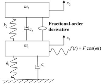
The model of fractional-order Voigt type DVA is shown in Fig. 1, which consists of the primary system and a damped DVA . The fractional-order element is put between the primary system and the DVA, which is in parallel with the spring and damper of the DVA. In vibration engineering, the fractional-order element may be arbitrary viscoelastic material and its force could be modelled as:
where and are the displacement of the primary system and the DVA, is the -order derivative of to with the fractional coefficient () and the fractional order (). There are several definitions for fractional-order derivative, and under some conditions they are equivalent. Here the Caputo’s definition is adopted for simplicity:
where is the Gamma function satisfying . In the fractional-order derivative, the initial condition is very important [36-38]. However, the steady-state responses are more meaningful in vibration engineering and both types of the derivatives will lead to the same steady-state solutions. Accordingly, the objective will be focused on the steady-state solution in the rest parts of this paper.
According to Newtonian second law, the motion equation could be established as:
where , , , , , are the masses, linear stiffness coefficients, and linear viscous damping coefficients of the primary system and DVA respectively. and are the amplitude and frequency of the external excitation.
Using the following parametric transformation:
Eq. (2) becomes:
Fig. 1The model of fractional-order DVA
2.1. The analytical solution based on the averaging method
According to the averaging method, one can suppose Eq. (3) has the solution as:
where , are the generalized phases. By differentiating Eq. (4) to one can obtain:
Combining Eq. (3) and Eq. (4) with Eq. (5), one can get:
where:
Solving Eq. (6) with , , , as unknowns, one obtains:
Moreover, one could apply the standard averaging method to Eq. (7) in time interval [39-40], that means:
One could select the time terminal as if the integrands are periodic or if the integrands are aperiodic. Then Eq. (8) can be divided into the following types:
where:
Then the first part of Eq. (9) will become:
For the second part of Eq. (9), the integration region should be . Here is taken as an example, and the others could be solved similarly. In order to calculate this integration, two important formulae are introduced [29-31]:
According to Eq. (12), one can get the integral in Eq. (10b):
The detail derivation procedures are presented in Appendix A. Similarly, one can get:
Combining Eq. (13) with Eq. (11), one could obtain:
The steady-state system response is more meaningful. Letting the right part of Eq. (14) be zero and simplifying the equation, one can obtain:
The steady-state amplitudes , and phases , can be obtained by solving Eq. (15). Accordingly, one can get:
where:
Substituting the parameters with the original ones, Eq. (16) could be transformed into:
where:
Two new parameters and , defined as equivalent damping coefficient and the equivalent stiffness coefficient, can be introduced. Then Eq. (17) can be rewritten as:
where:
2.2. optimization of the DVA
The calculation will be very complicated if the primary system contains viscous damping, so that the primary system without damping is considered. One could suppose in the equivalent damping coefficient and the equivalent stiffness coefficient because the main object of optimization criterion is to reduce the maximum resonance amplitude of the primary system. Here the amplitude amplification factor is defined based on Eq. (18) and the parameters in Eq. (3):
where:
Considering the undamped primary system, namely , Eq. (19) can be:
According to the fixed-point theory, the amplitude of the primary system will pass through two fixed points independent of the damping ratio . Assuming the two to be equal when and , one can get:
One can find that there is no meaning if the right part of the equal sign is positive. Taking the negative one and simplifying the equation, one could obtain:
Solving Eq. (22), one can get:
2.2.1. The optimal equivalent frequency ratio
Substituting into respectively when , one can obtain:
Simplifying Eq. (24), one will get:
According to Eq. (23), one can obtain:
Comparing Eq. (25) with Eq. (26), one can get:
The optimal equivalent frequency ratio can be obtained by solving Eq. (27):
Substituting into , then the abscissas of the two fixed points can be obtained:
2.2.2. The optimal equivalent damping ratio
Substituting the optimal equivalent frequency ratio into , differentiating to , and equating the obtained slopes to zero at the two optimal equivalent frequency ratio, one could get the best equivalent damping ratio:
Based on Eq. (30), one could obtain an average value between the two given optimal equivalent damping ratios:
In order to determine the optimal equivalent stiffness and equivalent damping, the optimal frequency ratio and the optimal damping ratio are replaced by the equivalent stiffness and the equivalent damping. After simplification one could get:
The optimal fractional order and the fractional coefficient can be obtained by solving Eq. (32):
That means, the fractional-order element could replace the linear spring and damper simultaneously in optimization criterion, and reduce the maximum resonance amplitude of the primary system the same as traditional Voigt type DVA.
2.3. optimization of the DVA
optimization will be more desirable if the system is subjected to random excitation instead of harmonic excitation, because the object of this optimization criterion is to reduce the total vibration energy of the primary system over the whole-frequency range. It means the area under the amplitude-frequency curve of the primary system should be minimized.
The performance index is defined as follow for the optimization criterion:
where the symbol is statistical average, the symbol is the temporal averages, and is the uniform power spectrum density of the excitation force respectively. The mean square value of the displacement of the primary system is calculated by the following equation:
where is the amplitude amplification factor. Thus the performance index can be simplified as:
Based on the residue theorem, Eq. (36) will be:
where:
The performance index has a minimum value at a certain combination of and when the value of and is given. This condition is achieved when both the partial derivatives of with respect to and are zero. Considering the undamped primary system, one can get a pair of simultaneous equations after differentiation:
Eliminating for solving the functions, the equation about can be obtained:
The optimal equivalent tuning ratio can be obtained by solving Eq. (39):
Substituting into Eq. (38), the optimal equivalent damping ratio can be obtained as:
Replacing the parameters with the equivalent stiffness and the equivalent damping, one could get a pair of equations about and :
Solving the equations one can get the optimal fractional order and the fractional coefficient for optimization criterion:
That means, the fractional-order element could replace the linear spring and damper simultaneously in optimization criterion, and reduce the total energy of the primary system as traditional Voigt type DVA.
3. Numerical simulation and comparison
3.1. The comparison between the analytical and numerical solution
The numerical results are also presented to verify the precision of the analytical solution. Here the numerical formula presented in [17, 18] are adopted:
where is the sample points, is the sample step, is the binomial coefficient with the iterative relationship as:
The total computation time is selected as 400 s and the sample step is 0.001 s. The peak value of the later 50 s response is taken as the steady-state amplitude of the numerical results and the temporary response in frontal 350 s is omitted.
Based on the above optimized results, one could investigate the effect of the fractional-order parameters through the following four groups of parameters:
a) 0, .
b) 0, ,
c) 6000, ,
d) 6000, .
The other system parameters are selected as 1000, 100000, 0, 100, 1000000.
3.1.1. optimization criterion
According to Eq. (19) and Eq. (33), the analytical normalized amplitude-frequency curves of the primary system are plotted in Fig. 2 and denoted by the solid lines. The corresponding numerical results are also shown in Fig. 2, and denoted by the circles. From the figure it could be found that the two kinds of curves agree well, that means the approximately analytical solution is satisfactorily precise. Moreover, the similarity of those curves shows that all the analytical amplitudes remain almost the same no matter how the stiffness coefficient and damping coefficient changes. That means the fractional order and fractional coefficient can affect the dynamic system characteristics by affecting the equivalent stiffness and the equivalent damping coefficient. Even it could replace the linear spring and damper of DVA completely. This result is different from the traditional results where the fractional-order derivative was generally regarded as damping device only.
3.2. optimization criterion
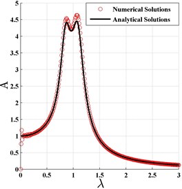
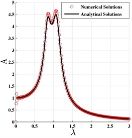
Based on the aforementioned system parameters, the normalized amplitude-frequency curves are plotted in Fig. 3 according to the optimal and in Eq. (43). It could also be found that the analytical solutions agree very well with the numerical results in optimization case.
Fig. 2The normalized frequency response curve based on H∞ optimization criterion
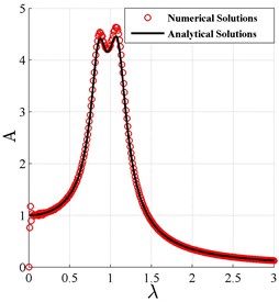
a)0, 0
b)0, 100
c)6000, 0
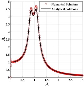
d)6000, 100
Fig. 3The normalized frequency response curve based on H2 optimization criterion
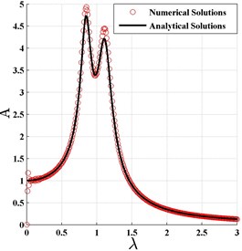
a)0, 0
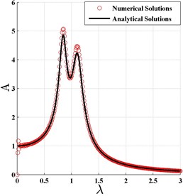
b)0, 100
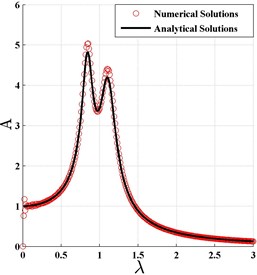
c)6000, 0

d)6000, 100
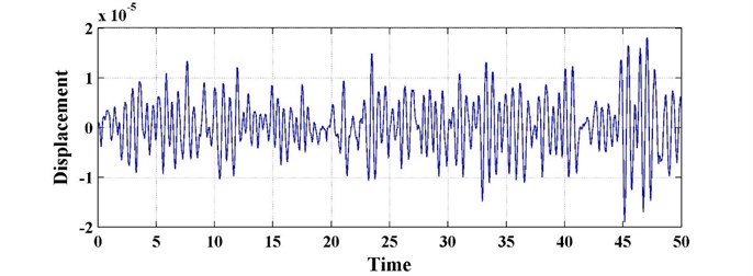
To study more realistic situation, 50 s random excitation are constructed, which is composed of 5000 random numbers with normal distribution. The excitation is normalized so that it is with mean value 0 and variance 1. The time history of the random excitation is shown in Fig. 4. When there is no fractional-order derivative in the Voigt type DVA, the time history of the primary system is given in Fig. 5. Here the optimum parameters are 8686 and 285, which are obtained according to reference [15]. For comparison the time histories of the primary system with the fractional-order DVA for the above different system parameters are presented in Fig. 6 to Fig. 9. The variances of the primary system in the above five systems are summarized in Table 1.
Table 1The variances of the displacement of the primary system
The integer-order DVA | The fractional-order DVA | ||||
0, 0 | 0, 100 | 6000, 0 | 6000, 100 | ||
Variances | 3.929e-11 | 2.8434e-11 | 2.8632e-11 | 2.8348e-11 | 2.8577e-11 |
Fig. 4The time history of random excitation
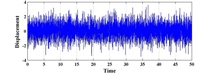
From the Figs. 4-9 and Table 1 it could be concluded that the fractional-order DVA can not only reduce the peak displacement of the primary system ( optimization criterion), but also reduce the total energy of the primary system in the whole-frequency range ( optimization criterion).
Fig. 5The time history of the primary system without fractional-order derivative (k2= 8686, c2= 285)
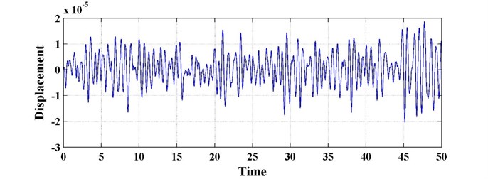
Fig. 6The time history of the primary system with fractional-order derivative (k2= 0, c2= 0)
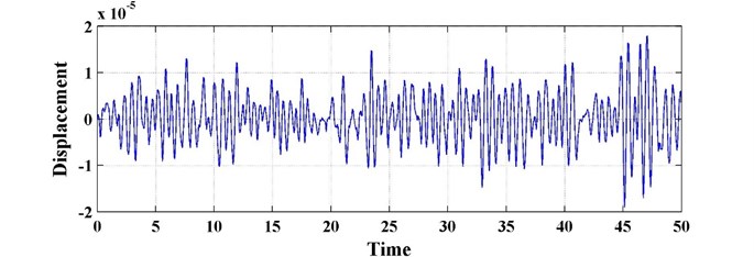
Fig. 7The time history of the primary system with fractional-order derivative (k2= 0, c2= 100)

Fig. 8The time history of the primary system with fractional-order derivative (k2= 6000, c2= 0)
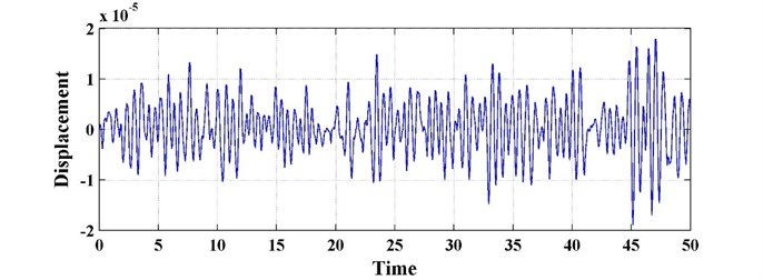
Fig. 9The time history of the primary system with fractional-order derivative (k2= 6000, c2= 100)
3.3. The comparison with the Voigt type DVA
In order to verify the performance of the fractional-order DVA, the comparison between the fractional-order and the traditional integer-order Voigt type DVA is presented in this subsection.
The amplification factor of the integer-order Voigt type DVA is:
According to the reference [4], the optimal parameters of Voigt DVA for the optimization criterion is , , .
The comparison of the fractional-order and the traditional integer-order Voigt type DVA is shown in Fig. 10. The parameters and are all selected as 0 in the fractional-order DVA so as to find out the effect of fractional-order derivative on the system clearly.
Similarly, one can choose the following parameters according to the existing literature [15] for the optimization criterion , , .
Fig. 10The comparison of the fractional-order and integer-order Voigt type DVA for H∞ optimization criterion
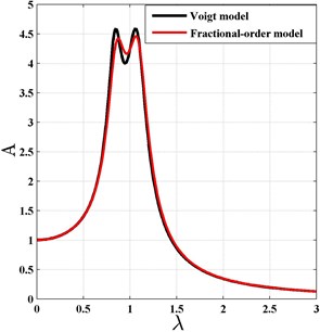
Fig. 11The comparison of the fractional-order and integer-order Voigt type DVA for H2 optimization criterion
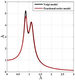
To observe the effect of the fractional-order derivative, one can also select and to be zero. The comparison results are shown in Fig. 11. From Fig. 10 and Fig. 11, it could be found that in the two cases the amplitude-frequency curves of the fractional-order DVA agree well with those of the integer-order DVA, even when the linear stiffness and damping coefficients of the fractional-order DVA equal zero. That means the fractional-order derivative has a very good substitution for the stiffness and damping elements of DVA. The results also prove the correctness of the concept of equivalent stiffness and damping coefficients presented in references [29-31].
4. Conclusion
The optimization of the fractional-order DVA is studied in this paper, and the optimal fractional order and fractional coefficient are obtained for the and optimization criteria. The comparisons of the approximately analytical solutions with the numerical solutions certify the satisfactory precision of the approximately analytical solutions. The comparisons with the integer-order DVA show that the fractional-order derivative can almost replace the linear stiffness and linear damping element, which may make the dynamical system much simpler. As the fractional-order derivative can accurately model many viscoelastic materials for vibration control engineering, the linear spring and damping elements may be replaced by one fractional-order element. These results may be very useful to design or revise vibration control device in engineering. Of course, it is important to study the replacement in engineering practice, which may be the next study object.
References
-
Frahm H. Device for Damping Vibrations of Bodies. U.S. Patent, No. 989958, 30 October 1909.
-
Ormondroyd J., Den Hartog J. P. The theory of the dynamic vibration absorber. ASME Journal of Applied Mechanics, Vol. 1928, Issue 50, 7, p. 9-22.
-
Hahnkamm E. The damping of the foundation vibrations at varying excitation frequency. Ingenieur Archiv, Vol. 1932, 4, p. 192-201.
-
Brock J. E. A note on the damped vibration absorber. ASME Journal of Applied Mechanics, Vol. 13, Issue 4, 1946, p. 284.
-
Nishihara O., Asami T. Close-form solutions to the exact optimizations of dynamic vibration absorber (minimizations of the maximum amplitude magnification factors). ASME Journal of Vibration and Acoustics, Vol. 124, 2002, p. 576-582.
-
Crandall S. H., Mark W. D. Random Vibration in Mechanical Systems. Academic Press, New York, 1963.
-
Iwata Y. On the construction of the dynamic vibration absorbers. Japan Society of Mechanical Engineers, Vol. 820, Issue 8, 1982, p. 150-152.
-
Asami T. Optimum design of dynamic absorbers for a system subjected to random excitation. JSME International Journal, Vol. 34, Issue 2, 1991, p. 218-226.
-
Yamaguchi H. Damping of transient vibration by a dynamic absorber. Transactions of the Japan Society of Mechanical Engineers Series C, Vol. 54, Issue 499, 1988, p. 561-568.
-
Ioi T., Ikeda K. On the dynamic vibration damped absorber of the vibration system. Bulletin of The Japan Society of Mechanical Engineers, Vol. 21, Issue 151, 1978, p. 64-71.
-
Randall S. E., Halsted D. M., Taylor D. L. Optimum vibration absorbers for linear damped systems. ASME Journal of Mechanical Design, Vol. 103, 1981, p. 908-913.
-
Thompson A. G. Optimum tuning and damping of a dynamic vibration absorber applied to a force excited and damped primary system. Journal of Sound and Vibration, Vol. 77, Issue 3, 1981, p. 403-415.
-
Warburton G. B. Optimal absorber parameters for various combinations of response and excitation parameters. Earthquake Engineering and Structural Dynamics, Vol. 10, 1982, p. 381-401.
-
Nishihara O., Matsuhisa H. Design and tuning of vibration control devices via stability criterion. Japan Society Mechanical Engineering, Vol. 97, Issue 10, 1997, p. 165-168.
-
Asami T., Nishihara O., Baz A. M. Analytical solutions to H∞ and H2 optimization of dynamic vibration absorbers attached to damped linear systems. ASME Journal of Vibration and Acoustics, Vol. 124, 2002, p. 284-295.
-
Asami T., Nishihara O. Closed-form exact solution to H∞ optimization of dynamic vibration absorbers application to different transfer functions and damping systems. ASME Journal of Vibration and Acoustics, Vol. 125, Issue 3, 2003, p. 398-405.
-
Oldham K. B., Spanier J. The Fractional Calculus Theory and Applications of Differentiation and Integration to Arbitrary Order. Academic Press, New York, 1974.
-
Podlubny I. Fractional Differential Equations. Academic Press, London, 1999.
-
Petras I. Fractional-Order Nonlinear System. Higher Education Press, Beijing, 2011.
-
Mandelbrot B. B. Les Objets Fractals: Forme, Hasard et Dimension. Flammarion, Paris, 1975.
-
Machado J. A. T., Galhano A. M. S. Fractional dynamics: a statistical perspective. ASME Journal of Computational and Nonlinear Dynamics, Vol. 3, Issue 2, 2008, p. 021201
-
Li G., Zhu Z., Cheng C. Dynamical stability of viscoelastic column with fractional derivative constitutive relation. Applied Mathematics and Mechanics, Vol. 22, Issue 3, 2001, p. 294-303.
-
Wang Z., Hu H. Stability of a linear oscillator with damping force of fractional order derivative. Science China Physics, Mechanics and Astronomy, Vol. 53, Issue 2, 2010, p. 345-352.
-
Wang Z., Du M. Asymptotical behavior of the solution of a SDOF linear fractionally damped vibration system. Shock and Vibration, Vol. 18, 2011, p. 257-268.
-
Rossikhin Y. A., Shitikova M. V. Application of fractional derivatives to the analysis of damped vibrations of viscoelastic single mass systems. Acta Mechanica, Vol. 120, 1997, p. 109-125.
-
Cao J., Ma C., Xie H., Jiang Z. Nonlinear dynamics of Duffing system with fractional order damping. ASME Journal of Computational and Nonlinear Dynamics, Vol. 5, 2010, p. 041012
-
Sheu L. J., Chen H. K., Chen J. H., Tam L. M. Chaotic dynamics of the fractionally damped Duffing equation. Chaos, Solitons and Fractals Vol. 32, 2007, p. 1459-1468.
-
Wahi P., Chatterjee A. Averaging oscillations with small fractional damping and delayed terms. Nonlinear Dynamics, Vol. 38, 2004, p. 3-22.
-
Shen Y. J., Yang S. P., Xing H. J. Dynamical analysis of linear single degree-of-freedom oscillator with fractional-order derivative. Acta Physica Sinica, Vol. 61, Issue 11, 2012, p. 110505.
-
Shen Y. J., Yang S. P., Xing H. J., Ma H. X. Primary resonance of Duffing oscillator with two kinds of fractional-order derivatives. International Journal of Non-Linear Mechanics, Vol. 47, 2012, p. 975-983.
-
Shen Y. J., Yang S. P., Xing H. J., Gao G. S. Primary resonance of Duffing oscillator with fractional-order derivative. Communications in Nonlinear Science and Numerical Simulation, Vol. 17, 2012, p. 3092-3100.
-
Chen L., Hu F., Zhu W. Stochastic dynamics and fractional optimal control of quasi integrable Hamiltonian systems with fractional derivative damping. Fractional Calculus and Applied Analysis, Vol. 16, Issue 1, 2013, p. 189-225.
-
Chen L. C., Zhu W. Q. Stochastic jump and bifurcation of Duffing oscillator with fractional derivative damping under combined harmonic and white noise excitations. International Journal of Non-linear Mechanics, Vol. 46, Issue 12, 2011, p. 1324-1329.
-
Chen L. C., Li H. F., Li Z. S., Zhu W. Q. First passage failure of single-degree-of-freedom nonlinear oscillators with fractional derivative. Journal of Vibration and Control, Vol. 19, Issue 14, 2013, p. 2154-2163.
-
Chen L. C., Wang W. H., Li Z. S., Zhu W. Q. Stationary response of Duffing oscillator with hardening stiffness and fractional derivative. International Journal of Non-Linear Mechanics, Vol. 48, Issue 1, 2013, p. 44-50.
-
Achar N., Lorenzo C. F., Hartley T. T. Initialization and the Caputo Fractional Derivative. NASA John H. Glenn Research Center at Lewis Field Report, 2003.
-
Ortigueira M. D., Coito F. J. Initial conditions: what are we talking about? 3rd IFAC Workshop on Fractional Differentiation and its Applications, Ankara, Turkey, 2008.
-
Sabatier J., Merveillaut M., Malti R., Oustaloup A. On a representation of fractional order systems: interests for the initial condition problem. 3rd IFAC Workshop on Fractional Differentiation and its Applications, Ankara, Turkey, 2008.
-
Burd V. Method of Averaging for Differential Equations on an Infinite Interval: Theory and Applications. Taylor and Francis Group, 2007.
-
Shen Y. J., Zhao Y. X., Yang S. P., Xing H. J. A revised averaging method and general forms of approximate solution for nonlinear oscillator with only polynomial-type displacement nonlinearity. Journal of Vibroengineering, Vol. 16, Issue 4, 2014, p. 1864-1876.
Cited by
About this article

The authors are grateful to the support by National Natural Science Foundation of China (No. 11372198), the Cultivation Plan for Innovation Team and Leading Talent in Colleges and Universities of Hebei Province (LJRC018), the Program for Advanced Talent in the Universities of Hebei Province (GCC2014053), and the Program for Advanced Talent in Hebei Province (A201401001).
Yongjun Shen presented the whole structure of the article. Yongjun Shen and Haibo Peng wrote the draft manuscript. Shaofang Wen, Shaopu Yang, and Haijun Xing helped to improve the quality of the article in the preparation procedure.
