Simulation of spectrum-correspondent accelerogram by using artificial neural networks

1. Introduction

Among different seismic analysis methods of structures, dynamic analysis methods including spectrum analysis and time history analyses display a relatively high accuracy. The advantage of the former introduced in 1962 is the application of spectrum determined through so many earthquake records. The method was simple and compatible to the calculation capacity of that time. Furthermore, the obtained results relied on a set of earthquake records, but not a single accelerogram. Regarding current improvements in computers’ hardware and software, this method should nowadays be substituted with more accurate time history analysis method that can model non-linear behavior of structures [1]. However, the time history method relies on the selected earthquake records and the results vary from one record to another. In other words, a shortcoming of this method is the scarcity or the lack of records matching the geophysical and geotechnical conditions of the intended area. Therefore, researchers have attempted to generate appropriate accelerograms by simulation methods. A number of methods have been proposed for generating and simulating earthquake ground motions, including methods of Preumont [2], Fan and Ahmadi [3], Mukherjee and Gupta [4], Boore [5], Suarez and Zafarani et al. [6], Gavin and Dickinson [7], Zentner et al. [8], Rezaeian and Kiureghian [9], Soghrat et al. [10], Yamamoto and Baker [11], Rezaeian et al [12].

From another point of view, each record differs from others regarding PGA, frequency content, duration, etc. moreover, a single accelerogram cannot be considered as the representative of a set of accelerograms. Regarding the fact that each spectrum is obtained from a set of records, the respective accelerogram may be considered as the representative of the record set. Therefore, in this research it is attempt to obtain accelerograms corresponding to a design spectrum with similar characteristics of the recorded accelerograms of the area.

Several researchers have attempted to develop new methods for producing artificial earthquake records by the use of artificial intelligence methods. Using artificial neural networks, Ghaboussi and Lin [13] introduced a novel method for generating artificial accelerograms. In this method, at first, the accelerograms are compressed by Fourier transform function. The network is then trained to relate the response spectrum values to the compressed Fourier transform accelerogram values using a feed forward neural network. Lee and Han [14] introduced neural-network-based models for producing artificial earthquake and response spectra. Also, several neural-network-based models have been developed in an attempt to replace traditional processes to predict earthquake parameters of an area. Lin and Ghaboussi [15] suggested using stochastic neural networks to generate artificial accelerograms corresponding with a response spectrum. Sirca and Adeli [16] suggested a new method of simulating artificial earthquake accelerograms based on counterpropagation neural networks and wavelet packet transform. Using wavelet transforms and principal component analyses, Rajasekaran et al. [17] proposed five neural network-based models for generating artificial earthquake records and response spectra. Using neural networks, Ghaffarzadeh and Izadi [18] proposed a simulation technique generating artificial spatially varying seismic ground motions. Using wavelet theory and radial basic function neural networks, Amiri and Bagheri [19] suggested producing one artificial accelerogram compatible with the response spectrum. In order to predict peak ground acceleration Günaydın Kemal and Ayten [20] introduced a method based on feed-forward back-propagation, radial basis function and generalized regression neural networks. Using eight mathematically computed parameters known as seismicity indicators, Adeli and Panakkat [21] proposed a probabilistic neural network for the prediction of the magnitude of the largest earthquake in a pre-defined future time period in a seismic region using. In an attempt to produce more artificial earthquake accelerograms from, available data compatible with the specified response spectra or the design spectra, Amiri et al. [22] introduced a method based on wavelet packet transform and stochastic neural networks. Using artificial neural network and wavelet packet transform Asdi et al. [23] presented a numerical method for the decomposition of artificial earthquake records consistent with any arbitrarily specified target response spectra requirements. In order to generate spectrum-compatible near-field artificial earthquake accelerograms, Amiri et al. [24] introduced a new methodology based on particle swarm optimization, wavelet packet transform techniques, and multilayer feed-forward neural networks. Employing the previously recorded strong-motion data and machine-learning techniques, Alimoradi and Beck [25] developed a new method of data-based probabilistic seismic hazard analysis, and ground motion simulation.

Computing the spectrum from an accelerogram is a forward problem while determining an accelerogram from its spectrum is an inverse problem. It should be mentioned that a great deal of information is lost in gaining from the accelerogram to its response spectrum. This inverse problem, thus, does not have a single solution, and the accelerogram are not determined solely from their response spectrum. Therefore, the learning capabilities of generalized regression neural network are proposed in this article for the simulation of accelerograms from the spectrum. There are two reasons for the use of the response spectrum as the input. First, expression of the response spectrum related to an earthquake record requires much fewer data than that required for the expression of accelerogram of that earthquake. This would decrease the number of the input data in each sample, which would in turn lead to an increase in the capability of the neural network simulation. Moreover, the design spectrum representing the mean (or mean plus standard deviation) of the response spectra of the earthquake records in one type of soil in an area. It would be possible to obtain accelerogram corresponding to the design spectrum in the case of neural network training with the response spectrum.

In this study, generalized regression neural network is used in order to simulate artificial accelerograms. Having valid and correctly-measured data is an essential instrument for training purposes of artificial neural network. Also predictions are performed with a higher level of certainty using valid information. The accelerograms from Iran Strong Motion Network (some events in both horizontal directions of North-South, and East-West) are utilized for neural network training and testing. The response spectrum is used as the input for the training and the corresponding accelerogram as the output. After the achievement of the desired conformation, the accelerogram corresponding to the design spectrum of Iranian Building Seismic Design Code (standard 2800 [26]) are computed by simulating network. The proposed method has the advantage of high speed in record simulation, and smaller number of data needed for network training compared to other methods.

2. Training and testing sets

The final purpose of the simulation is to generate corresponding design spectrum records. Therefore, Earthquakes with various PGA, various epicentral distances, and various magnitude; in both horizontal directions are used for training and testing purposes. Training the simulating network requires records compatible with the seismicity condition of the intended area. In this study, such data are provided from Iran Strong Motion Network for soil type II of standard 2800 (with shear wave velocity of 375$<V_s<$750) in two components of North-South and East-West. The response spectrum is used as the input to the network, and the corresponding accelerogram is used as the output. After network training, the design spectrum for soil type II of standard 2800 is considered as input to the network, and corresponding accelerogram is simulated by network. Some features of events which are used as the training and testing set, including the name of station, occurrence date, PGA, latitude, longitude, epicentral distance, magnitude in each event and Vs30 (average soil shear wave velocity in the upper 30 meters below the ground surface) in each station are shown in Table A1 of Appendix. These events have been recorded on the Iranian Strong Motion Network of the Building and Housing Research Center (BHRC). This network consists of more than 1000 stations including three-component accelerographs in different active seismic regions of Iran [27].

Recorded accelerograms of various events, as well as accelerograms of each event in various stations have different time durations. Regarding simulating neural network limitations, an equal duration is allocated for all accelerograms by adding some zeroes to the end of records. Events employed in this study generally have strong motion durations of 20 to 30 seconds. To this end, the duration of records is extended to 30 seconds. Since the time interval between acceleration data in records ($∆t$) equals 0.02 seconds, each record includes 1500 data. The pseudo-acceleration response spectra ($S_a$) of the accelerograms are calculated in period domain of 0.02-3 seconds and with time intervals ($∆T_n$) of 0.02 seconds. Each spectrum contains 150 data, and the damping ratio ($\zeta$) is assumed 5 % for all the response spectra. All records are normalized to their awn PGA for the training of the network. As a result, the PGA of all records is 1, and the pseudo-acceleration spectrum values start from 1.

3. Generalized regression neural network

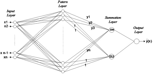
The generalized regression neural network (GRNN) was first presented by Specht [28]. Unlike the back propagation method, it does not require a repetitive training procedure. Drawing the function estimate directly from the training data, it approximates any arbitrary function between the input and output vectors. Moreover, the estimation error decreases as the training set increases in size, with only mild restrictions on the function. Like the standard regression techniques, the GRNN is used for estimating continuous variables. It is related to the radial basis function network and, is based on a standard statistical technique known as kernel regression. The GRNN is made up of four layers: the input layer, the pattern layer, the summation layer, and the output layer (Fig. 1). Each input unit in the input layer corresponds to an individual process parameter. The input layer is completely connected to the pattern layer. In this second layer, each unit represents a training pattern, and its output is a measure of the distance of the input from the stored patterns. Each pattern layer unit is connected to the two neurons in the summation layer- SW- and SU-summation neurons. The sum of the weighted outputs of the pattern layer is calculated by the SW-summation neuron; whereas the unweighted outputs of the pattern neurons are computed by the SU-summation neuron. The connection weight between the $i$th neuron in the pattern layer and the SW-summation neuron is $y_i$, which is the target output value corresponding to the $i$th input pattern. For SU-summation neuron is that of unity. The output of each S-summation neuron layer is simply divided by that of each SU-summation neuron (by the output layer) [29].

By definition, the most probable value for $y$ is estimated through the regression of a dependent variable $y$ on an independent variable $x$ - given $x$ and a training set. The regression method would minimize the mean-squared error (MSE) of the estimated value of $y$ (MSE). The GRNN is a method for the estimation of the joint probability density function (pdf) of $x$ and $y$ with the presence of merely a training set. The system is perfectly general since the pdf is achieved from the data with no preconception about its form.

Fig. 1Schematic framework of GRNN

If $f\left(x,y\right)$ shows the known joint continuous pdf of a vector random variable, $x$, and a scalar random variable, $y$, the conditional mean of $y$ given $X$ (also called the regression of $y$ on $X$) is given by:

When the density $f\left(x,y\right)$ is not known, it should be estimated from a sample of observations of $x$ and $y$. This equation is an estimator of $E\left[y\left|X\right.\right]$. The probability estimator $\widehat{f}(X,Y)$ is based upon sample values $X_i$ and $Y_i$ of the random variables $x$ and $y$, where $n$ is the number of sample observations and $p$ is the dimension of the vector variable $x$:

The probability estimate $\widehat{f}(X,Y)$ has a physical interpretation that it assigns a sample probability of width $\zeta$ for each sample $X_i$ and $Y_i$, and the probability estimate is the sum of these sample probabilities [28]. Defining the scalar function $D_i^2$:

and the mentioned integration having been performed, the following is achieved:

The estimate $\widehat{Y}\left(X\right)$ is shown as a weighted average of all the observed values-$Y_i$- in which the $\zeta$ is called the spread. The optimal value of spread is experimentally determined. It should be mentioned that all units in the pattern layer possess the same single spread in conventional GRNN applications in conventional GRNN applications in conventional GRNN applications in conventional GRNN applications [30]. The GRNN performance is controlled only by the spread factor during the training. In order to obtain the best prediction performance, various spreads were tried in the present study.

The GRNN has the advantages of fast learning and convergence to the optimal regression surface with the increase in the number of samples [31]. Another advantage of the GRNN is that it provides sparse data in a real-time environment. Since the regression surface can instantly be defined everywhere, even with just one sample [32].

4. The methodology suggested for record simulation

This study aims at presenting a new method to generate artificial accelerograms which have a response spectrum close to a specified response spectrum used as the input of the neural network (based on generalized regression neural network). In addition, the produced accelerogram from a given response spectrum should also have the characteristics like the group of accelerograms which is utilized in of the neural network training.

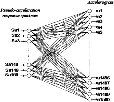
This method attempts to expand a generalized regression neural network which takes discretized ordinates of the pseudo-acceleration response spectrum of accelerogram as input, and the values of each accelerogram are used as the output. GRNN is a powerful function approximation technique based on statistical learning theory. The method provides excellent generalization performance while still being able to capture complex relationships in the input data. The framework of the final simulating machine is shown in Fig. 2. The network consists of 150 input neurons and 1500 output neurons. Among the recorded earthquakes in BHRC, 120 records consisting of 60 events in two components are selected for training and testing purposes (Table A1 of Appendix).

Fig. 2Framework of the simulating neural network

Earthquake records are time series with so many parameters; therefore, their comparison should be done employing various parameters (there is not a single parameter to compare records). Anderson introduced a method on the basis of quantitative scores [33]. The method can be used to evaluate the conformation of the synthetic records with the recorded ones. Anderson suggested using a suite of measurements. The characteristics scored are the peak acceleration, peak velocity, peak displacement, Arias intensity, the integral of velocity squared, Fourier spectrum and acceleration response spectrum on a frequency-by-frequency basis, the shape of the normalized integrals of acceleration and velocity squared, and the cross correlation. The parameters are illustrated as $C_1$, $C_2$,... and $C_{10}$, respectively. The averaging of the scores on the ten individual criteria $C_1$ to $C_{10}$ yields the average of all of these scores, $C_{ave}$. The comparison of each characteristic is conducted on a scale from 0 to 10, with 10 giving perfect agreement. Scores for each parameter are averaged to yield an overall quality of fit. A score below 4 indicates a poor fit, a score of 4-6 is a fair fit, a score of 6 to 8 represents a good fit, and a score over 8 is an excellent fit. The method would be used for evaluating the simulated records, and determining the parameters and the optimal framework of the network.

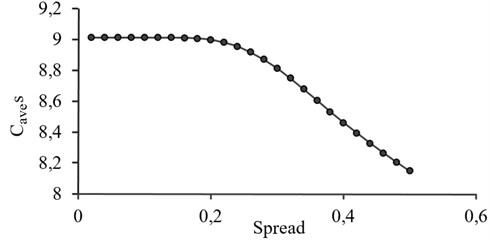
Pseudo-acceleration spectra, pseudo-velocity spectra, or displacement spectra can be used as the input to the network. To find the best input, the abovementioned spectra in the order mentioned are applied as the input which yields the $C_{ave}$ of the records as 9.01, 8.77 and 7.25, respectively. This shows that applying pseudo-acceleration spectra gives the best compatibility. The number of neurons in the input and output layers cannot be changed; because they are the number of data used to define the spectrum (150) and accelerograms (1500), respectively. Therefore, the spread factor is the only parameter which can be changed to find the optimum framework. For this, different spread factors are applied and $C_{ave}$s of the generated data are determined. As shown in Fig. 3 the spread factor smaller than 0.1 gives the greatest $C_{ave}$, therefore the spread factor is selected as 0.1.

Fig. 3The effect of spread constant on GRNN performance

5. Results of the simulations

Results of the record simulations are presented for two categories of training data-sets and testing data-sets in this section. 120 sets of data (the accelerograms, response spectra for both horizontal components of the earthquakes) form 60 events have been prepared, including 80 validation sets (previously applied to train the simulating neural network) and 40 testing sets. In order to increase network performance and accurate the simulation, as shown in all figures, accelerograms and response spectra are normalized to PGA values.

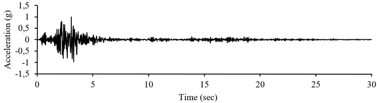
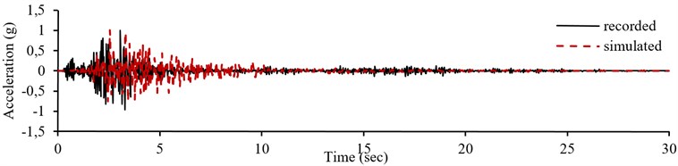
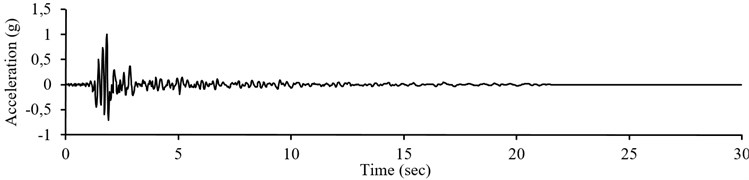
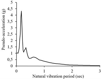
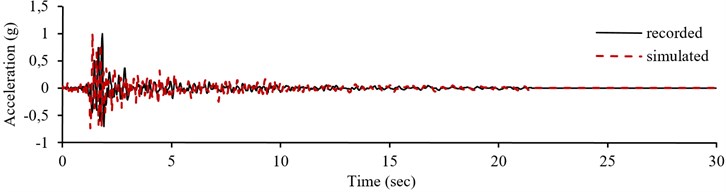
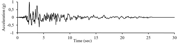
For the first instance, the data set of record number 17 (Table A1 of Appendix) from validation setts, in East-West component is presented in Fig. 4, including accelerogram (Fig. 4(a)) and the pseudo-acceleration response spectrum (Fig. 4(b)). The achieved accelerogram of the simulation is shown in Fig. 4(c), and compared with the recorded ones.

The correlation of the simulated records with the recorded ones is evaluated based on a method proposed by Anderson [33]. The comparison of recorded and simulated accelerogram for E-W component of record number 17 (Fig. 4) from validation sets is illustrated in Table 1. As shown, all parameters, $C_1$ to $C_{10}$, and their averages $C_{ave}$ for simulated record is greater than 8 which is indicating that the simulated accelerograms an excellent fit of the main recorded accelerograms.

Fig. 4Normalized recorded accelerogram, pseudo-acceleration response spectrum and simulation result of record number 17 in E-W component from training sets

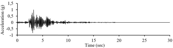
a) Normalized recorded accelerogram

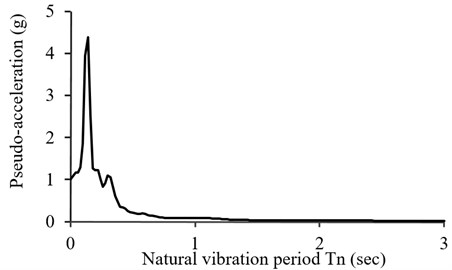
b) Normalized pseudo-acceleration response spectrum

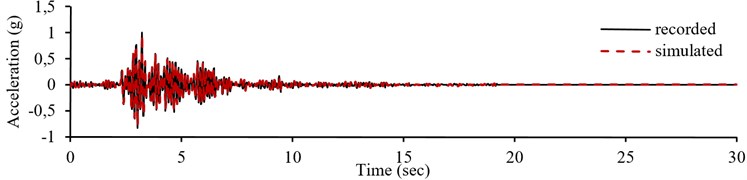
c) Comparison of recorded and simulated accelerograms

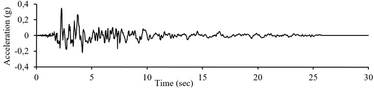
For another instance, the testing set data is focused; the neural network is evaluated for E-W component of record number 24 in Fig. 5. Normalized accelerogram of record number 24 (Table 1 of Appendix) is illustrated in Fig. 5(a). The pseudo acceleration response spectrum of the record shown in Fig. 5(b) is considered as the neural network input. The results of the simulation are presented in Fig. 5(c). The simulated accelerogram is compared with the recorded ones by Anderson parameters in Table 2. Moreover, Fig. 6 shows the same procedure for another record of testing set, record number 40 in E-W component Figs. 6(a) and 6(b) contain the recorded accelerograms of E-W component of record number 40 and its response acceleration spectrum. The results of the simulation are presented in Fig. 6(c). Table 3 illustrates evaluation of the simulated records, compared with the recorded ones.

The results (in Table 2 and Table 3) indicate good conformity between the simulated accelerograms and the recorded ones even when provided with new data. As shown, most of the parameters score are in the range of 8 to 10. The average of these parameters (Cave) is close to 8, confirming good fitting of the simulation. This represents a good accuracy of the simulating neural network even when provided with new data. In Table 2 and Table 3, the least score among Anderson’s proposed parameters belongs to the parameter $C_{10}$. This parameter is actually the indicator of the cross correlation between the recorded earthquakes and the simulated records and considers time differences between the simulated and recorded accelerograms [33]. The parameter will have small values if there is a little time delay between the simulated and recorded accelerogram.

Fig. 5Normalized recorded accelerogram, pseudo-acceleration response spectrum and simulation result of record number 24 in E-W component from testing sets

a) Normalized recorded accelerogram

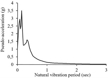
b) Normalized pseudo-acceleration response spectrum as input to simulating neural network

c) Comparison of recorded and simulated accelerograms

6. Generating accelerograms from the design spectrum

Regarding good generalizability of the simulating neural network, and in an attempt to produce accelerograms for the intended soil type, the design spectrum of seismic design code, is used in this phase as the input for the network.

Recorded of Table A1 of appendix and their correspondent spectra are used respectively as output and input for training the simulating neural network. As mentioned before, all of these records are recoded on soil type II (with Vs30 of 375 to 750 m/sec). The pseudo acceleration design spectrum of standard 2800 for soil profile type II (with $∆T_n$ of 0.02 sec, with time periods of 0.02-3 seconds and a damping ratio of 5 %) is considered as the neural network inputs (Fig. 7(a)). For this spectrum it is assumed that the design base acceleration (A) is 1, regarding that all records and response spectra employed in network training are normalized on PGA value. The output of the simulating network is presented in Fig. 7(b). As can be seen, PGA value of the simulated accelerogram is approximatively 1.

Fig. 6Normalized recorded accelerogram, pseudo-acceleration response spectrum and simulation result of record number 40 in E-W component from testing sets

a) Normalized recorded accelerogram

b) Normalized pseudo-acceleration response spectrum as input to simulating neural network

c) Comparison of recorded and simulated accelerograms

According to the levels of seismicity of the intended area, the achieved accelerogram should be multiplied by the design base acceleration ($A$); the simulated records for soil type II in an area with the relative seismic hazard of very high is illustrated in Fig. 7(c) (which is determined by multiplying 0.35 to Fig. 7(b)). Iran is divided into four zones including very high, high, moderate, and low seismicity, with design base acceleration of 0.35, 0.3, 0.25, and 0.2, respectively [25]. The obtained accelerograms can be used in linear and nonlinear time-history analyses of structures, on soil type II. Similar procedure can be carried out for other soil types and corresponding design acceleration spectrum, in presence of having sufficient suitable accelerogram on the same soil type, for training the simulating neural network.

Fig. 7The output of the simulating network

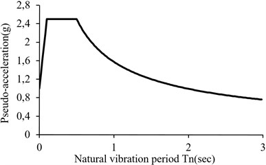
a) Design spectrum of Iranian code of practice for seismic resistance design of buildings for soil profile type II

b) Simulated accelerogram corresponding to the design spectrum

c) Simulated records corresponding to the design spectrum in an area with the relative seismic hazard of very high ($A=$0.35)

7. Conclusion

In this paper, a new methodology is proposed to simulate artificial spectrum-correspondent accelerogram. The time history analysis method has a better precision compared to other seismic analysis of structures, and is capable of modeling non-linear behavior of structures. A disadvantage of the method is the scarcity or lake of appropriate earthquake records indicative of the features of probable earthquake in an area in which the structure is constructed. To this end, a simplified artificial neural network -based approach is suggested- Generalized Regression Neural Network (GRNN). Recorded accelograms of Iranian Strong Motion Network are used to train the artificial neural network. The response spectrum is used as the input for the neural network, and the corresponding accelerogram as the output. Comparison of the recorded and simulated accelerograms by Anderson method indicates high learning capability of the GRNN in simulating seismic ground motions. The design spectrum is in fact an average of the available response spectra in an area. If a record compatible with the design spectrum is presented, it can be the best record for time history analyses of structures in the area. Finally, compatible accelerograms of the design spectrum, suggested in Iranian code of practice for seismic resistant design of buildings (standard 2800), is simulated with the proposed neural network.

The network can be utilized for the simulation of records compatible with the design spectrum in other soil types if appropriate sufficient accelerograms for the training of network for the intended soil types are supplied. In addition, the method is capable of generating records compatible with other seismic codes if appropriate training data are provided.