Abstract
When utilizing conventional regular focus point distributions to define a relatively large source region, Fourier-based deconvolution beamforming, an attractive acoustic source identification technique, would suffer from some limitations: 1) significantly deteriorative location and quantification accuracy for sources away from the center of the focus region; 2) pronounced sidelobe contaminations. The arch-criminal is the assumption that the point spread function (PSF) is definitely shift-invariant over the entire focus region fails to be satisfied well. This paper focuses on remedying these limitations for two-dimensional (2D) acoustic source identification. First and foremost, a novel focus point generation approach is introduced, which can generate unconventional irregular 2D focus point distributions tending to make PSF more shift-invariant. Additionally, a sidelobe suppression approach is suggested. Effects of these approaches are examined both with computer simulations and experimentally. This study provides the feasibility of using Fourier-based deconvolution beamforming to accurately and efficiently identify acoustic sources in a relatively large region.
1. Introduction
Beamforming with planar microphone arrays has become a popular technique for acoustic source identification [1]. Results of the traditional Delay and sum (DAS) beamforming [1-4] are affected by poor spatial resolution and severe sidelobe contaminations. The distortion is triggered by the fact that DAS’s output can be regarded as the sum of each source’s pressure contribution to array center multiplied with a corresponding PSF, whereas the PSF is not an ideal Kronecker delta function. In recent years, a deconvolution-based refined beamforming that can reduce effects of the poor spatial resolution or the sidelobes to insignificance has been developed. Deconvolution approach for the mapping of acoustic sources (DAMAS) [5, 6], nonnegative least-squares (NNLS) [7], Richardson-Lucy (RL) [8-11], sparsity constrained DAMAS [12], covariance matrix fitting [12], DAMAS2 [13], Fourier-based NNLS [7] and Fourier-based RL [7] are all quintessential deconvolution algorithms. Thereinto, the last three are all built on a fast Fourier transform, and corresponding beamforming is collectively termed as Fourier-based deconvolution beamforming.
Expressing DAS’s output as a convolution of pressure contribution and PSF in spatial domain and using a fast Fourier transform to perform the multiplication in wavenumber domain, Fourier-based deconvolution beamforming enjoys incomparable efficiency superiority. It is due to the pleasurable feature that the technique exerts a tremendous fascination on scholars and engineers. A host of application cases associated with aircrafts, vehicles, wind turbines and some other objects has been reported [14-16]. Nevertheless, when identifying sources in a relatively large region that is defined by a conventional regular focus point distribution, Fourier-based deconvolution beamforming would be burdened with two obvious limitations. One is significantly deteriorative location and quantification accuracy for sources away from the point where a shift-invariant PSF is defined, the other one is pronounced sidelobe contaminations. The arch-criminal is the fact that the technique intrinsically assumes PSF to be definitely shift-invariant over the entire focus region, namely depending only on the relative position between the focus point and the source and not on the individual positions [7, 13, 17, 18], whereas the real PSF under the conventional case is merely approximately shift-invariant in a reasonably small region, and seriously shift-variant in a large one. As an unfavorable consequence, Fourier-based deconvolution beamforming with a conventional regular focus point distribution can only obtain promising results for sources in a very limited region.
Some scholars have endeavored to alleviate these limitations. Ehrenfried et al. [7] proposed an embedded approach where DAMAS2 and Fourier-based NNLS were embedded in an outer iteration to take the variation of PSF into account. Suzuki [19] introduced a PSF weakly varying in space by expanding the real PSF in a Taylor series and retaining up to the second-order terms and used it in DAMAS2. Both of the two approaches work at the expense of increased computational cost. Especially, the embedded approach will even consume several days to process a complete engineering data. Additionally, Xenaki et al. [20-21] as well as Dougherty [13] took over the three-dimensional (3D) coordinate transformation technique applied in underwater acoustic vision to ameliorate the 3D shift-invariance of PSF and further improve the 3D acoustic source identification quality. This approach scarcely sacrifices the original efficiency superiority, just needing to generate focus points arranged in a set of concentric hemispherical surfaces. As a matter of fact, in a multitude of cases, beamforming with planar microphone arrays is in demand to identify sources in a 2D region parallel to the array plane. Accordingly, it is indispensable to probe into new approaches that can not only effectively but also efficiently remedy these limitations and thus enhance the 2D acoustic source identification. This paper focuses on this issue. Main highlights are: (1) a novel focus point generation approach is introduced, which can generate unconventional irregular 2D focus point distributions tending to improve the 2D shift-invariance of PSF dramatically. Fourier-based deconvolution beamforming with the unconventional irregular focus point distribution is capable of substantially increasing the detection accuracy in terms of the source pressure contribution and location. (2) A sidelobe suppression approach is suggested, whose incorporation enables Fourier-based deconvolution beamforming with the unconventional irregular focus point distribution to further enjoy strong sidelobe suppression capability. (3) An appropriate value range is explored and recommended for the key parameter in the sidelobe suppression approach.
The remainder of this paper is organized as follows: in Section 2, principles of beamforming are presented, including DAS and Fourier-based deconvolution. Thereafter, Section 3 introduces the generation approach of unconventional irregular 2D focus point distributions and researches the shift-invariance improvement of PSF. Subsequently, in Section 4, a sidelobe suppression approach is suggested and researched. Moreover, based on simulations of some given acoustic sources, performance comparisons of the Fourier-based deconvolution beamforming under different conditions are demonstrated. Next, Section 5 is devoted to validate correctness of the simulation conclusions and effectiveness of these approaches in practical applications by experiments. Finally, conclusions are summarized in Section 6.
2. Principles of beamforming
2.1. DAS: Delay and sum
Beamforming involves capturing the sound field with an array of microphones and post-processing the array measurements by an algorithm that scans a focus region for acoustic sources. DAS is the commonly used algorithm, which processes the data in a constructive way giving a reinforced output if the focus position is the correct source location, otherwise in a destructive way giving an attenuated output. The DAS response of a planar array comprising microphones focused at the point , denoted as , can be written as:
where is the cross-spectral matrix of the sound pressure signals captured by microphones, is an unity matrix with all elements equal to 1, is the focus column vector with 1, 2,…, being the serial number of the microphones, and [20-22]. The superscript “” and “” represent the transposition and the conjugation respectively. Element is defined by:
where denotes the position of the th microphone, is the imaginary unit, and is the wavenumber for frequency and the speed of sound .
For incoherent sources, the cross-spectral matrix equals the sum of elementary matrices related to each one of the sources. Denoting by and the position and the pressure contribution to array center of a source respectively, we arrive at:
where is a function of , describing the map resulting from a unit-pressure-contribution point source at This map is referred to as the PSF. In the expression of , denotes the sound propagation column vector of the source. Its element can be obtained by replacing in Eq. (2) with . In the ideal case the PSF would be a Kronecker delta function, and the DAS response would reveal the locations and the pressure contributions of sources within the focus region directly. Unfortunately, this is never the case since the finite size of the array and the discrete pattern of microphones impose poor resolution and give rise to sidelobes.
2.2. Fourier-based deconvolution
Considering focus points and letting , and denote the DAS response vector, the PSF matrix and the pressure contribution distribution vector respectively, a linear system of equations can be yielded:
Deconvolution attempts to solve Eq. (4) for , aiming at attenuating effect of the PSF and rendering explicit source maps. In deconvolution process, the DAS response can be calculated directly based on Eq. (4), but that is computationally heavy since the PSF matrix is in general too huge to be acquired in a short time. Alternatively, it can also be calculated indirectly based on a computationally advantageous Fourier transform method. Foremost, introduce a function and assume a property reflected in the form:
which means depends only on the difference between the focus position and the source location . Such a PSF is called shift-invariant since its shape does not change with source location and the overall beam pattern can be simply shifted in space. Then, insert Eq. (5) into Eq. (3) to lead to:
which corresponds to a discrete convolution. Finally, make use of the convolution theorem to obtain:
where the operators “”, “” and “” stand for the convolution, the direct and the inverse Fourier transforms, respectively. Obviously, the shift-invariance of PSF is a key issue for Fourier-based deconvolution beamforming. Often, the function is acquired by considering the source centered at the focus region [7, 13, 15-18].
Fourier-based NNLS deconvolution algorithm is taken as an example to perform simulations and experiments in this paper, which extracts the pressure contribution distribution vector by minimizing a defined quadratic residual function. A gradient-project procedure is often utilized, which solves the NNLS problem by searching along the negative gradient direction of the quadratic residual function in space iteratively [7, 16-18]. Initialize the iteration index, , and use an estimation of , to start. The iteration cycle from solution to consists of the following procedures:
1. Compute the residual :
2. Calculate the negative gradient of the quadratic residual function in space as:
by defining a shift-invariant mirrored PSF in advance. The relationship holds for :
3. Use vector to define a search path through the current position , whose components can be obtained by:
where denotes the negative gradient component of the quadratic residual function in the direction of .
4. Compute the auxiliary value :
5. Stack up the residual and the auxiliary value at each focus point to form a residual vector and an auxiliary vector respectively. Estimate the optimal step factor by:
6. Determine components in the new solution by:
3. Shift-invariance improvement through an unconventional irregular 2D focus point distribution
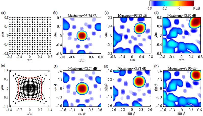
Layout of beamforming measurement is illustrated by Fig. 1, where an array of microphones represented by the star is lying in the plane and the focus region is placed parallel to the array at a distance of . After dimension parameters denoted by , , and have been set for the focus region, conventional beamforming divides it with equal space along and directions respectively to form a regular focus point distribution, as shown in Fig. 2(a). PSFs under this case are plotted in Fig. 2(b)-(d) with each one corresponding to a source location. In each figure, a wide mainlobe together with plenty of sidelobes occurs. Apparently, both the mainlobe shape and the sidelobe structure change with the source location. Moreover, relative to Fig. 2(b), changes in Fig. 2(c) are more serious than that in Fig. 2(d). These phenomena demonstrate that under the conventional regular 2D focus point distribution, the shift-invariance of the PSF is poor, especially for sources far apart from each other. That will inevitably impede the ability of Fourier-based deconvolution beamforming to identify acoustic sources.
Fig. 1Layout of beamforming measurement
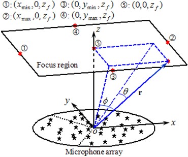
Unlike conventional beamforming, this paper presents a novel focus point generation approach. As shown in Fig. 1, two angles, and , are defined for the position vector . Thereinto, is the angle between the vector and its projection to the plane, and similarly, is the angle between the vector and its projection to the plane. According to simple geometrical considerations:
where , and are the Cartesian coordinates of the vector . For points in the focus region, locates in the range of to where keeps monotonic, so do . As a consequence, any focus point can be determined uniquely by where is a constant. Denoting by and the minimum and maximum value of , and similarly, and the minimum and maximum value of in the focus region, we arrive at that and appear at and respectively by geometrical analysis. These four positions are numbered as 1, 2, 3 and 4 successively in Fig. 1. Therefore:
Fig. 2PSFs at 3000 Hz of sources at different locations ((b), (c), (d)) under (a) the conventional regular 2D focus point distribution and ((f), (g), (h)) under (e) the unconventional irregular one
The novel approach uniformly divides to and to to generate focus points. According to the relationship shown in Eq. (15), the Cartesian coordinates and of the unconventional focus point can be calculated by:
Fig. 2(e) depicts the focus points generated by the novel approach, whose distribution is irregular and part of which lies outside the focus region (encircled by the dash line). PSFs under this case are plotted in Fig. 2(f)-(h), with the abscissa and the ordinate being and respectively. Apparently, both the mainlobe shape and the peak are consistent irrespectively of the source location, even though the sidelobe structure still changes, declaring that the PSF components in mainlobe have nearly kept shift-invariant with regard to and . A detailed theoretical demonstration can be found in the Appendix. To sum up, compared with the conventional regular 2D focus point distribution, the unconventional irregular one is capable of improving the shift-invariance of the PSF dramatically, which is expected to enhance the 2D acoustic source identification with Fourier-based deconvolution beamforming.
4. Simulations
In order to examine the superiority of the unconventional irregular 2D focus point distribution, simulations are conducted using a 36-element sector wheel array with a diameter of 0.65 m, whose geometrical setup is shown in Fig. 1. Detailed process is: (1) assume a specific source pressure contribution distribution, including source position, source pressure contribution and frequency; (2) calculate the sound pressure signal captured by each microphone and their cross-spectra; (3) set a focus region that encompasses all the sources, and generate the conventional and unconventional focus point distribution according to the approaches described in Section 3; (4) focus each point with DAS algorithm shown by Eq. (1) and map acoustic sources; (5) reconstruct and map the pressure contribution distribution with Fourier-based NNLS deconvolution shown by Eq. (8)-(14). Here, the focus region covers an area of 1.6 m×1.6 m and is at a distance of 1 m from the array. The grid space is 0.025 m×0.025 m for the conventional regular focus point distribution. The total number of iterations is specified as 200 in deconvolution.
4.1. Single source
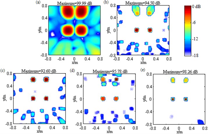
Table 1 lists contour maps of single source identification, where each column corresponds to a source location, and from Column 1 to Column 4, the distance of the source to the center of the focus region is growing. All the sources have a pressure contribution of 100 dB and a frequency of 3000 Hz. In order to compare with each other clearly, output values in each map are scaled to dB by referring to the maximum one and the display dynamic ranges are all set as 18 dB, namely from 0 dB to –18 dB. Meanwhile, the maximum output value is labeled on the top of each map, which has been scaled to dB by referring to 2.0×10⁻⁵ Pa. Maps in Row 1 illustrate DAS’s output, which indicate the source locations successfully, but are characterized by wide mainlobes and plenty of sidelobe contaminations. Maps in Row 2 depict the pressure contribution distribution reconstructed by Fourier-based NNLS deconvolution with the conventional regular 2D focus point distribution, where even though mainlobes have been narrowed and partial sidelobes have been wiped up, some limitations still emerge. For instance, in the maps in Column 2-4, the mainlobe peaks are created at (0.275, 0.275, 1) m, (0.45, 0.45, 1) m and (0.8, 0.8, 1) m, deviating from the true source locations approximately by 0.04 m, 0.07 m and 0.14 m respectively. Besides, all the mainlobes are affected by a trailing that will mislead someone into thinking another source exists. Only the source at (0.1, 0.1, 1) m is located correctly, as shown in the map in Column 1. Conversely, with the unconventional irregular 2D focus point distribution, Fourier-based NNLS deconvolution is capable of not only creating the mainlobe peak at the true source location but also enjoying a narrow and neat mainlobe, whether the source is close to or away from the center of the focus region, as shown in maps in Row 3. Additionally, Table 2 lists calculation errors of the pressure contribution for the three methods. Thereinto, DAS calculates the pressure contribution as its mainlobe peak, which can be demonstrated by substituting Eq. (A8) into Eq. (3), while Fourier-based NNLS deconvolution calculates the pressure contribution as the linear superposition of the output values over its mainlobe [7, 18]. It is apparent that both DAS and Fourier-based NNLS deconvolution with the unconventional irregular 2D focus point distribution can detect each source’s pressure contribution within no more than 0.23 dB discrepancy, whereas for Fourier-based NNLS deconvolution with the conventional regular 2D focus point distribution, the error deteriorates with the increase of the distance of the source to the center of the focus region and the maximum one reaches up to 4.18 dB. In conclusion, with a conventional regular 2D focus point distribution, Fourier-based deconvolution beamforming can neither locate nor quantify the source away from the center of the focus region effectively. As stated in [20-21], only sources in an angular region of no more than 18° off the center axis of microphone array (-axis) can be identified. The unconventional irregular 2D focus point distribution breaks through this limitation, enabling Fourier-based deconvolution beamforming to successfully locate and quantify the source in a significantly enlarged region. The valid opening angle can reach 45°, which means a closer location distance from the microphone array to the source plane is allowed to identify sources in the same region.
Table 1Contour maps showing simulations of single sources at different locations at 3000 Hz
 | |||||
Source locations | (0.1, 0.1, 1) m | (0.3, 0.3, 1) m | (0.5, 0.5, 1) m | (0.7, 0.7, 1) m | |
DAS |  | 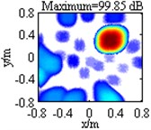 | 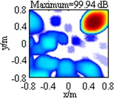 | 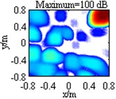 | |
Fourier-based NNLS deconvolution with different 2D focus point distributions | Regular | 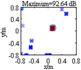 | 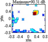 | 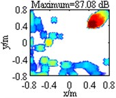 | 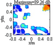 |
Irregular | 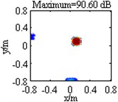 | 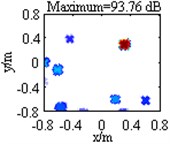 | 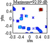 | 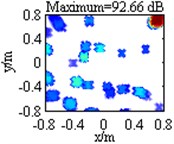 | |
Table 2Calculation errors of the pressure contribution
Source locations | (0.1, 0.1, 1) m | (0.3, 0.3, 1) m | (0.5, 0.5, 1) m | (0.7, 0.7, 1) m | |
DAS | 0.23 dB | 0.15 dB | 0.06 dB | 0 dB | |
Fourier-based NNLS deconvolution with different 2D focus point distributions | Regular | 0.21 dB | 1.40 dB | 3.32 dB | 4.18 dB |
Irregular | 0.15 dB | 0.03 dB | 0.01 dB | 0.01 dB | |
As shown in Row 2-3 in Table 1, contour maps obtained with both of the two Fourier-based NNLS deconvolution methods still suffer from pronounced disturbing sidelobes, especially when the source is away from the center of the focus region. To delve deeper, we extract the maximum sidelobe level (MSL) from each map and list them in Table 3. Obviously, it is for each source that the MSL resulting from Fourier-based NNLS deconvolution with the conventional regular 2D focus point distribution is higher than that from DAS, and particularly for the source at (0.5, 0.5, 1) m, the former is even 4.51 dB higher than the latter. Compared to the conventional focus point distribution, the unconventional one enables Fourier-based NNLS deconvolution to outperform slightly. Nevertheless, the corresponding MSL is still higher than that from DAS for the source at (0.1, 0.1, 1) m or (0.7, 0.7, 1) m, indicating that Fourier-based deconvolution beamforming fails to suppress sidelobes effectively, even if the unconventional irregular 2D focus point distribution is utilized. This can be attributed to the fact that the PSF is not absolutely shift-invariant. As clarified in Section 3 and Appendix, under the unconventional irregular 2D focus point distribution, only the PSF components in mainlobe nearly keep shift-invariant, while the others are still distinctly shift-variant. High-level sidelobes will confuse the acoustic source identification results. Considering that sidelobes are invariably weaker than mainlobes, this paper attempts to suppress sidelobes by setting all components in the reconstructed pressure contribution distribution vector below a certain threshold to zero in each iteration, where the threshold is computed as the largest component minus an introduced parameter of decibel. Further, considering that sidelobes in general become weaker with the increase of iteration, the parameter can be updated in an increase way during the iteration. This paper initialize 0.05 dB and utilize a linear increase way. The value after iterations is calculated as:
where is the total number of iterations and is referred to as the upper limit on . In the iteration, the components in the solution are reset as in the following way:
where stands for the largest component in . Stack up all to form a new solution vector and take it as the input in the iteration. In order to examine the validity of the sidelobe suppression approach, simulations are conducted using the source shown in Column 3 in Table 1 and with the parameter being specified as 33 dB. The resulting maps corresponding to the conventional and the unconventional focus point distribution are respectively depicted in Fig. 3(a) and Fig. 3(b). In both of them, the mainlobe peak is created at the true source location, namely (0.5, 0.5, 1) m, and the linear superposition of the output values over the mainlobe has a fairly small deviation from the true pressure contribution, concretely 0.35 dB and 0.30 dB separately. A comparison of these phenomena and the corresponding ones shown in Table 1 and Table 2 declares that the incorporation of the sidelobe suppression approach effectively improves the source location and quantification accuracy of Fourier-based deconvolution beamforming with the conventional regular 2D focus point distribution, and hardly affects the intrinsic high accuracy of Fourier-based deconvolution beamforming with the unconventional irregular 2D focus point distribution. Additionally, Fig. 3(a) exhibits good sidelobe suppression in the lower left corner but high sidelobe contaminations around the mainlobe. Its MSL is still up to –6.28 dB. Conversely, Fig. 3(b) is totally free of sidelobes in the display dynamic range, where the MSL is only –20.90 dB that is 8.50 dB lower than the one resulting from Fourier-based NNLS deconvolution with the unconventional irregular 2D focus point distribution but not with the sidelobe suppression approach (presented in Row 3 Column 3 in Table 3) and 9.87dB lower than the one from DAS (presented in Row 1 Column 3 in Table 3). Therefore, a conclusion can be drawn that the sidelobe suppression approach is fairly effective when combined with the unconventional irregular 2D focus point distribution. The last but not the least, under the condition that a 2.5 GHz Intel(R) Core(TM) i5-2450 M CPU is used to run the Matlab programs, it takes 3.95 s, 4.06 s, 4.18 s and 4.30 s in sequence to obtain the maps in Row 2 Column 3 in Table 1, Row 3 Column 3 in Table 1, Fig. 3(a) and Fig. 3(b). The approximate consistency demonstrates that the proposed approaches barely sacrifice the efficiency superiority of the original Fourier-based deconvolution beamforming.
Table 3MSLs extracted from the contour maps in Table 1
Source locations | (0.1,0.1,1) m | (0.3,0.3,1) m | (0.5,0.5,1) m | (0.7,0.7,1) m | |
DAS | –13.30 dB | –11.39 dB | –11.03 dB | –10.21 dB | |
Fourier-based NNLS deconvolution with different 2D focus point distributions | Regular | –11.70 dB | –9.83 dB | –6.52 dB | –8.09 dB |
Irregular | –13.02 dB | –12.65 dB | –12.40 dB | –9.88 dB | |
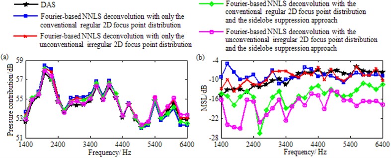
is a key parameter in the above-mentioned sidelobe suppression approach. In order to determine its appropriate range, simulations are conducted using Fourier-based NNLS deconvolution with the unconventional irregular 2D focus point distribution. Taking a source with a location at (0.5, 0.5, 1) m and a pressure contribution of 100 dB as an example, Fig. 4(a)-(c) give out the curves of main acoustic source identification performance indices vs. at 3000 Hz, 4000 Hz and 5000 Hz. These indices include number of focus points in mainlobe, calculation error of pressure contribution and MSL. Thereinto, the first one is utilized to measure spatial resolution. The more the number is, the wider the mainlobe is, the poorer the spatial resolution is. Three figures exhibit consistent phenomena: (1) the number of focus points in mainlobe does not exceed 11 within the entire range of , which only occupies 0.26 % of the total number; (2) the calculation error of pressure contribution is relatively large and remains unchanged when 25 dB, decreases progressively when , and converges to a very small value when 40 dB; (3) the MSL is negative infinity when 30 dB (not drawn in the figures), and basically increases with the growth of when 30 dB. These phenomena can still be achieved when some parameters such as the frequency, the number of iterations and the source location are changed. They indicate: (1) no matter what value is, excellent spatial resolution can be obtained; (2) to calculate the pressure contribution accurately, should be as large as possible; (3) to suppress sidelobes effectively, should be as small as possible. Taking the contradictory relationship between the latter two into consideration, this paper recommends the range of 32 dB to 35 dB for , which can provides a good compromise between pressure contribution calculation on one side and sidelobe suppression on the other side, as shown in Fig. 4(a)-(c).
Fig. 3Contour maps showing simulations of single source identification at 3000 Hz after the application of Fourier-based NNLS deconvolution with different 2D focus point distributions: a) conventional regular one; b) unconventional irregular one. In both of them, the sidelobe suppression approach is incorporated
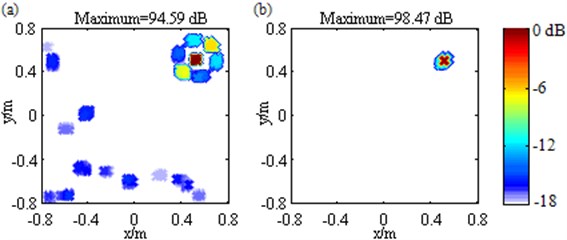
Fig. 4Main acoustic source identification performance indices vs. Rmax: a) at 3000 Hz; b) at 4000 Hz; c) at 5000 Hz and vs. frequency: d) for a Rmax of 33 dB
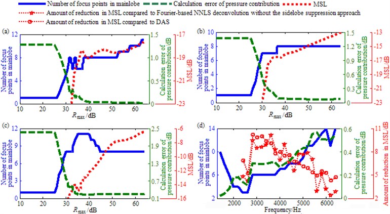
Moreover, Fig. 4(d) draws the curves of number of focus points in mainlobe, calculation error of pressure contribution and amount of reduction in MSL compared to Fourier-based NNLS deconvolution without the sidelobe suppression approach or DAS vs. frequency for a of 33 dB. It is apparent that within the entire frequency range, both the number of focus points in mainlobe and the calculation error of pressure contribution are fairly small, not exceeding 14 and 0.6 dB respectively. Besides, the amount of reduction in MSL is positive, and particularly positive infinite for frequencies below 2200 Hz (not drawn in the figure), meaning that the MSL is suppressed effectively. As a consequence, when the value of falls into the recommended range, it is at each frequency that Fourier-based deconvolution beamforming with the unconventional irregular 2D focus point distribution and the sidelobe suppression approach can enjoy excellent spatial resolution, high pressure contribution calculation accuracy as well as good sidelobe suppression. These conclusions provide guidance for the appropriate assignment of .
4.2. Multiple sources
In this section, performance comparisons of Fourier-based deconvolution beamforming under different conditions are demonstrated for multiple sources. Four sources are simultaneously considered, among which two are close to the center of the focus region, being at (–0.2, 0, 1) m and (0.2, 0, 1) m respectively, and the other two are away, being at (–0.2, 0.6, 1) m and (0.2, 0.6, 1) m respectively. The same pressure contribution of 100 dB and frequency of 3000 Hz are assumed for these sources. First, DAS algorithm is applied and the resulting map is shown in Fig. 5(a), where four mainlobe peaks are created at the true source locations and separately equal to 99.89 dB, 99.82 dB, 99.95 dB and 99.99 dB, meaning that the sources are located and quantified successfully, but the mainlobes are wide and with a maximum level of –7.08 dB, the sidelobes almost contaminate the whole region except mainlobes. Next, Fourier-based NNLS deconvolution with only the conventional regular 2D focus point distribution is applied and the reconstructed pressure contribution distribution is shown in Fig. 5(b). Obviously, for the sources at (–0.2, 0, 1) m and (0.2, 0, 1) m, two narrow and neat mainlobes appear. A further analysis finds that not only the mainlobe peaks are exactly created at the true source locations but also the linear superposition of the output values over each mainlobe only deviates by 0.1 dB from the true pressure contribution. Different from that, for the sources at (–0.2, 0.6, 1) m and (0.2, 0.6, 1) m, both of the mainlobes are affected by a trailing, both of the mainlobe peak positions deviate from the true source locations by about 0.08 m, and both of the calculated pressure contributions have an error of up to 2.57 dB. Again, the limitation that with only a conventional regular 2D focus point distribution, Fourier-based deconvolution beamforming can neither locate nor quantify sources away from the center of the focus region effectively is verified. It can be eliminated by an unconventional irregular 2D focus point distribution, as demonstrated in Fig. 5(c) where every mainlobe enjoys not only a narrow and neat shape but also a peak created at the true source location, and all the calculated pressure contributions are extremely close to the true one, only with an error of 0.07 dB, 0.05 dB, 0.01 dB and 0.02 dB in turn. Furthermore, even though Fig. 5(b) and Fig. 5(c) exhibit some sidelobe suppression compared to Fig. 5(a), many sidelobes still exist and the MSL reaches up to –9.79 dB and –10.17 dB respectively. With the aim of sweeping away sidelobes, the suggested sidelobe suppression approach is incorporated, with the parameter being specified as 33 dB. The resulting maps corresponding to the conventional and the unconventional focus point distribution are depicted in Fig. 5(d) and Fig. 5(e) respectively. Fig. 5(d) still suffers from many sidelobes and being –9.48 dB, the MSL is even higher than the one in Fig. 5(b) and Fig. 5(c), demonstrating that the combination of the conventional regular 2D focus point distribution and the sidelobe suppression approach fails to suppress sidelobes. Conversely, Fig. 5(e) exhibit only two sidelobes and the MSL is only –14.98 dB that is 7.90 dB, 5.19 dB, 4.81 dB and 5.50 dB lower than the one in Fig. 5(a), Fig. 5(b), Fig. 5(c) and Fig. 5(d) respectively, demonstrating that the combination of the unconventional irregular 2D focus point distribution and the sidelobe suppression approach is capable of suppressing sidelobes strongly. Besides, in both Fig. 5(d) and Fig. 5(e), for each source, a narrow and neat mainlobe appears, its peak is created at the true source location and the calculated pressure contribution has a fairly small error, meaning that all the sources are located and quantified successfully as well as resolved clearly. Specifically, the quantification errors are 0.10 dB, 0.09 dB, 0.15 dB and 0.35 dB in turn for these four sources in Fig. 5(d) and 0.21 dB, 0.14 dB, 0.17 dB and 0.16 dB in Fig. 5(e). To summarize, both the unconventional irregular 2D focus point distribution and the sidelobe suppression approach can enhance the identification of these multiple equal-pressure-contribution sources. Their combination brings the optimal performance, enabling Fourier-based deconvolution beamforming to not only locate and quantify each source successfully but also ameliorate spatial resolution and suppress sidelobe contaminations remarkably. Additionally, change the pressure contribution of the sources at (–0.2, 0, 1) m, (–0.2, 0.6, 1) m and (0.2, 0.6, 1) m into 98.75 dB, 103.01 dB and 96.99 dB in turn and keep the remaining one unchanged. Corresponding simulations are conducted and the resulting maps are depicted in Fig. 6. It presents similar phenomena with Fig. 5, indicating that Fourier-based deconvolution beamforming with the unconventional irregular 2D focus point distribution and the sidelobe suppression approach shown by Fig. 6(e) is optimal. This method correctly indicates all the source locations, remarkably narrows all the mainlobes, obtain all the pressure contributions within no more than 0.39 dB discrepancy, and almost removes all the sidelobes. Consequently, the unconventional irregular 2D focus point distribution and the sidelobe suppression approach also can enhance the identification of these multiple unequal-pressure-contribution sources.
Fig. 5Contour maps showing simulations of multiple sources identification at 3000 Hz after different post-processing techniques: a) DAS; b) Fourier-based NNLS deconvolution with only the conventional regular 2D focus point distribution; c) Fourier-based NNLS deconvolution with only the unconventional irregular 2D focus point distribution; d) Fourier-based NNLS deconvolution with the conventional regular 2D focus point distribution and the sidelobe suppression approach; e) Fourier-based NNLS deconvolution with the unconventional irregular 2D focus point distribution and the sidelobe suppression approach. The sources are equal-pressure-contribution
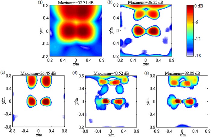
Changing the frequency of the sources shown in Fig. 5 into 1500 Hz, and conducting simulations, the resulting maps are depicted in Fig. 7. Fig. 7(a) shows that DAS generates four mutually fused mainlobes and some sidelobes no higher than –13.11 dB. This is due to its intrinsic poor-spatial-resolution and low-level-sidelobe characteristics at low frequencies. Fig. 7(b) follows same behavior as Fig. 5(b) and Fig. 6(b), namely that Fourier-based NNLS deconvolution with only the conventional regular 2D focus point distribution reconstructs the source locations and pressure contributions successfully as well as improves the spatial resolution effectively for the sources at (–0.2, 0, 1) m and (0.2, 0, 1) m, while fails to do that for the other two sources. A location error of up to 0.10 m and a quantification error of up to 2.33 dB come out for both of the sources at (–0.2, 0.6, 1) m and (0.2, 0.6, 1) m. In contrast to that, Fig. 7(c) demonstrates Fourier-based NNLS deconvolution with the unconventional irregular 2D focus point distribution is capable of not only reconstructing all the source locations and pressure contributions successfully but also ameliorating spatial resolution and suppressing sidelobes effectively. The removal behavior of sidelobes is vastly superior to the one shown in Fig. 5(c) and Fig. 6(c), which is due to DAS’s intrinsic low-level-sidelobe characteristic and PSF’s low shift-variance at low frequencies. The former is verified by Fig. 7(a) and the latter can be explained as following. Eq. (A2) attests the exponent is a key to determine . Apparently, the lower the frequency is, the smaller the wavenumber is, the weaker the amplification degree of the shift-variant part in becomes. As a result, the PSF enjoys low shift-variance at low frequencies, which makes the prerequisite of shift-invariant PSF in Fourier-based deconvolution beamforming to be fulfilled better. Finally, Fig. 7(d) and Fig. 7(e) present totally confusing results, which are strikingly different from the corresponding ones presented in Fig. 5 and Fig. 6. A lot of simulations have founded that when the mainlobes generated by DAS fuse with each other, the incorporation of the sidelobe suppression approach will result in confusion. Considering the characteristic that DAS’s mainlobe width is inversely proportional to frequency, the fusion phenomenon of mainlobes often occurs at low frequencies, however fortunately, in this case, only with the unconventional irregular 2D focus point distribution, Fourier-based deconvolution beamforming is capable of obtaining low-level sidelobes, as shown in Fig. 7(c), that is to say, the sidelobe suppression approach is really not needed. Additionally, it is worth noting that simulations shown in Figs. 5-7 are based on an assumption of incoherence, and same conclusions can also be achieved when the sources are assumed to be coherent. For sake of conciseness, corresponding contour maps are not given.
Fig. 6Contour maps showing simulations of multiple sources identification at 3000 Hz after different post-processing techniques: a) DAS; b) Fourier-based NNLS deconvolution with only the conventional regular 2D focus point distribution; c) Fourier-based NNLS deconvolution with only the unconventional irregular 2D focus point distribution; d) Fourier-based NNLS deconvolution with the conventional regular 2D focus point distribution and the sidelobe suppression approach; e) Fourier-based NNLS deconvolution with the unconventional irregular 2D focus point distribution and the sidelobe suppression approach. The sources are unequal-pressure-contribution
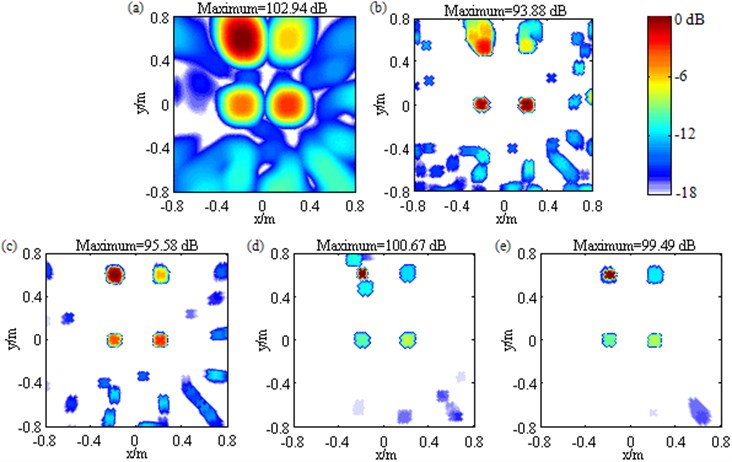
Fig. 7Contour maps showing simulations of multiple sources identification at 1500 Hz after different post-processing techniques: a) DAS; b) Fourier-based NNLS deconvolution with only the conventional regular 2D focus point distribution; c) Fourier-based NNLS deconvolution with only the unconventional irregular 2D focus point distribution; d) Fourier-based NNLS deconvolution with the conventional regular 2D focus point distribution and the sidelobe suppression approach; e) Fourier-based NNLS deconvolution with the unconventional irregular 2D focus point distribution and the sidelobe suppression approach
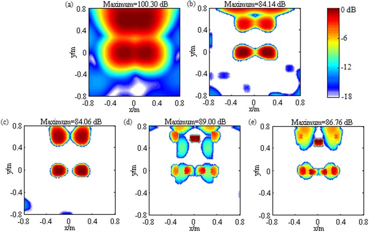
Fig. 8Sketch map of the experimental configuration
5. Validation experiments
With the purpose of validating correctness of the simulation conclusions and effectiveness of the unconventional irregular 2D focus point distribution as well as the sidelobe suppression approach in practical applications, a series of experimental measurements are performed in a semi-anechoic room. The configuration is depicted in Fig. 8. A sector wheel array with a diameter of 0.65 m and comprising 36 Brüel&Kjær Type 4958 microphones is adopted. Four loudspeakers excited by stationary white noises serve as acoustic sources, which are located at (–0.2, 0, 1) m, (0.2, 0, 1) m, (–0.2, 0.6, 1) m and (0.2, 0.6, 1) m respectively. Sound pressure signals received by microphones are acquired simultaneously by Brüel&Kjær 41-channel PULSE Type 3560D Data Acquisition System and then transferred to Brüel&Kjær PULSE LABSHOP Software where their cross-spectra are achieved. The sample frequency is 16384 Hz, Hanning windows is utilized, the overlap is 66.7 percent, the number of blocks is 64, each block has a length of 0.25 s, and the frequency resolution is 4 Hz. Eventually, DAS and various Fourier-based NNLS deconvolution methods are applied to map the source field and reconstruct the pressure contribution distribution by MATLAB programming. In accordance with simulations, the focus region is built to cover an area of 1.6 m×1.6 m, the conventional regular 2D focus point distribution is generated using a grid space of 0.025 m×0.025 m, the deconvolution methods perform 200 iterations, and the parameter is specified as 33 dB.
5.1. Single source
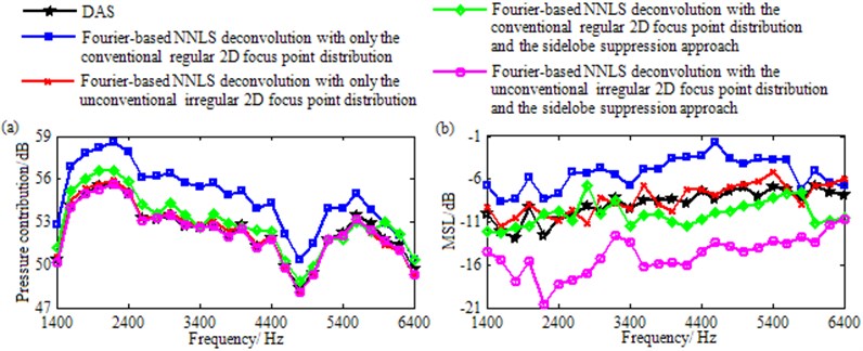
Fig.9 contains the contour maps at 3000 Hz for the measurement with only the loudspeaker at (–0.2, 0, 1) m excited. The loudspeaker is close to the center of the focus region. Fig. 9(a) illustrates DAS’s output. Fig. 9(b)-(e) depict the pressure contribution distribution reconstructed by Fourier-based NNLS deconvolution with, in sequence, only the conventional regular 2D focus point distribution, only the unconventional irregular 2D focus point distribution, the conventional regular 2D focus point distribution and the sidelobe suppression approach, and the unconventional irregular 2D focus point distribution and the sidelobe suppression approach. In each map, the mainlobe peak position coincides with the true source location. In Fig. 9(a), a mainlobe with a width of 0.4 m is exhibited. In Fig. 9(b)-(e), the mainlobe has been narrowed remarkably. Particularly in Fig. 9(d)-(e), the mainlobe width is only 0.05 m. Contour maps at other frequencies also present similar phenomena, demonstrating that whether with the conventional regular or the unconventional irregular 2D focus point distribution, Fourier-based deconvolution beamforming can accurately locate this loudspeaker source as well as ameliorate the spatial resolution, and when the sidelobe suppression approach is incorporated, the best spatial resolution is achieved. As described in Section 3, the mainlobe peak output by DAS reliably expresses the source pressure contribution. Fig. 9(a) shows the pressure contribution of this loudspeaker source is 54.37 dB, which can serve as a benchmark to measure the quantification accuracy of Fourier-based deconvolution beamforming. From Fig. 9(b) to Fig. 9(e), by linear superposition of the output values over the mainlobe, the pressure contribution is calculated as 55.16 dB, 55.10 dB, 54.81 dB and 54.81 dB respectively. All of them are in close proximity to 54.37 dB. Further, Fig. 10(a) gives out the curves of calculated pressure contribution vs. frequency for the five methods. Obviously, all the curves almost coincide, demonstrating that whether with the conventional regular or the unconventional irregular 2D focus point distribution and whether with the sidelobe suppression approach or not, Fourier-based deconvolution beamforming can successfully quantify this loudspeaker source. Additionally, in Fig. 9(a), plenty of sidelobes occur and the MSL is –10.41 dB. In Fig. 9(b) and Fig. 9(c), the sidelobes are lessened, but the MSL is grown to –7.06 dB and –7.57 dB respectively. Different from that, Fig. 9(d) exhibits only three sidelobes and the MSL is reduced to –15.44 dB, and Fig. 9(e) gets rid of sidelobes. Further, Fig. 10(b) gives out the curves of MSL vs. frequency. Obviously, the MSL resulting from DAS as well as Fourier-based NNLS deconvolution with only the conventional regular or the unconventional irregular 2D focus point distribution is highest, and the latter two methods even work worse than DAS at many frequencies. By comparison, the remaining two methods outperform distinctly. Particularly, Fourier-based NNLS deconvolution with the unconventional irregular 2D focus point distribution and the sidelobe suppression approach obtains the lowest MSL at all frequencies except 2600 Hz and 5000 Hz. These phenomena demonstrate that the incorporation of the sidelobe suppression approach can effectively remedy the drawback of failing to suppress and even growing sidelobes suffered by Fourier-based deconvolution beamforming with only the conventional regular or the unconventional irregular 2D focus point distribution, and the combination of the unconventional irregular 2D focus point distribution and the sidelobe suppression approach brings best suppression effect. To sum up, for the practical single source close to the center of the focus region, whether with the conventional regular or the unconventional irregular 2D focus point distribution, Fourier-based deconvolution beamforming is capable of locating and quantifying the source successfully as well as ameliorating spatial resolution effectively, the incorporation of the sidelobe suppression approach is capable of further ameliorating spatial resolution and suppressing sidelobe contaminations remarkably, and the combination of the unconventional irregular 2D focus point distribution and the sidelobe suppression approach brings optimal identification performance.
Fig. 9Contour maps showing identification results of a single loudspeaker source at 3000 Hz after different post-processing techniques: a) DAS; b) Fourier-based NNLS deconvolution with only the conventional regular 2D focus point distribution; c) Fourier-based NNLS deconvolution with only the unconventional irregular 2D focus point distribution; d) Fourier-based NNLS deconvolution with the conventional regular 2D focus point distribution and the sidelobe suppression approach; e) Fourier-based NNLS deconvolution with the unconventional irregular 2D focus point distribution and the sidelobe suppression approach. The source is located at (–0.2, 0, 1) m
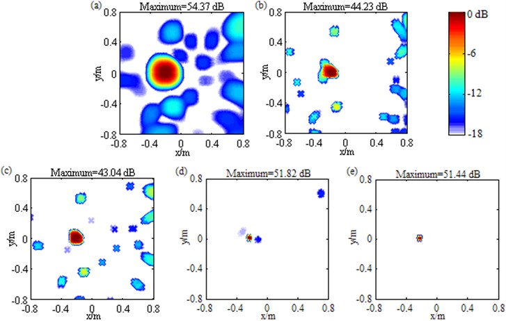
Fig. 10a) Calculated pressure contribution and b) MSL vs. frequency when the single loudspeaker source at (–0.2, 0, 1) m is identified
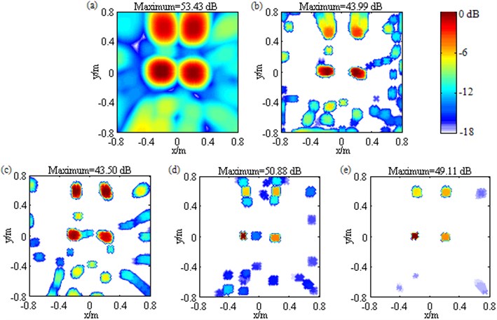
Following the layout in Fig. 9, Fig. 11 contains the contour maps at 3000 Hz for the measurement with only the loudspeaker at (0.2, 0.6, 1) m excited. The loudspeaker is away from the center of the focus region. Compared to Fig. 11(a), Fig. 11(b) possesses a slightly narrowed mainlobe. However regrettably, the mainlobe is affected by a trailing and its peak position, (0.2, 0.525, 1) m, deviates from the true source location by 0.075 m. Conversely, Fig. 11(c)-(e), particularly Fig. 11(d)-(e), all enjoy a narrow and neat mainlobe as well as a mainlobe peak position coinciding with the true source location. Contour maps at other frequencies also present similar phenomena, demonstrating that Fourier-based deconvolution beamforming with only the conventional regular 2D focus point distribution fails to locate this loudspeaker source accurately, whereas the other three methods can not only compensate for this failure but also ameliorate the spatial resolution, and when the sidelobe suppression approach is incorporated, the best spatial resolution is achieved. As shown in Fig. 11(a), the pressure contribution of this loudspeaker source is 53.44 dB. From Fig. 11(b) to Fig. 11(e), Fourier-based NNLS deconvolution calculates it as 56.38 dB, 53.68 dB, 54.29 dB and 53.47 dB in turn. They deviate from 53.44 dB by 2.94 dB, 0.24 dB, 0.85 dB and 0.03 dB respectively. Obviously, the quantification error suffered by Fourier-based NNLS deconvolution with only the conventional regular 2D focus point distribution (the first one) is significant, whereas the remaining three, especially the second and the fourth ones corresponding to the unconventional irregular 2D focus point distribution, are acceptable. The curves of calculated pressure contribution vs. frequency plotted in Fig. 12(a) further show that the rule holds for almost all frequencies, demonstrating that Fourier-based deconvolution beamforming with only the conventional regular 2D focus point distribution fails to quantify this loudspeaker source, whereas the other three methods also can compensate for this failure effectively, especially Fourier-based deconvolution beamforming with the unconventional irregular 2D focus point distribution.
Fig. 11Contour maps showing identification results of a single loudspeaker source at 3000 Hz after different post-processing techniques: a) DAS; b) Fourier-based NNLS deconvolution with only the conventional regular 2D focus point distribution; c) Fourier-based NNLS deconvolution with only the unconventional irregular 2D focus point distribution; d) Fourier-based NNLS deconvolution with the conventional regular 2D focus point distribution and the sidelobe suppression approach; e) Fourier-based NNLS deconvolution with the unconventional irregular 2D focus point distribution and the sidelobe suppression approach. The source is located at (0.2, 0.6, 1) m
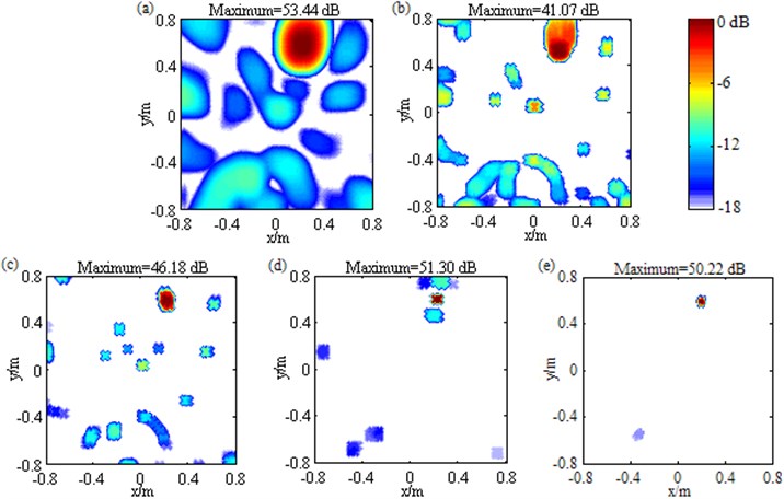
Additionally, it is apparent that Fig. 11(e) is much cleaner than the other maps, among which Fig. 11(a) suffers from plenty of sidelobes, Fig. 11(b) as well as Fig. 11(e) is affected by significantly grown MSL, and Fig. 11(d) is contaminated by high-level sidelobes near the mainlobe. The curves of MSL vs. frequency plotted in Fig. 12(b) further show that with a maximum of –1.76 dB that is even comparable to the mainlobe level, the MSL resulting from Fourier-based NNLS deconvolution with only the conventional regular 2D focus point distribution is highest within the entire frequency range, the ones from DAS and Fourier-based NNLS deconvolution with only the unconventional irregular 2D focus point distribution or with the conventional regular 2D focus point distribution and the sidelobe suppression method are tied for second, whereas the one from Fourier-based NNLS deconvolution with the unconventional irregular 2D focus point distribution and the sidelobe suppression approach is lowest. These phenomena demonstrates for this loudspeaker source, only the combination of the unconventional irregular 2D focus point distribution and the sidelobe suppression approach can enable Fourier-based deconvolution beamforming to suppress sidelobes effectively. To sum up, for the practical single source away from the center of the focus region, Fourier-based deconvolution beamforming with only the conventional regular 2D focus point distribution fails seriously in terms of source location, source quantification and sidelobe suppression, Fourier-based deconvolution beamforming with only the unconventional irregular 2D focus point distribution or with the conventional regular 2D focus point distribution and the sidelobe suppression approach can compensate for the first two failures, but still fails to suppress sidelobe, whereas Fourier-based deconvolution beamforming with the unconventional irregular 2D focus point distribution and the sidelobe suppression approach can compensate for all the failures, not only locating and quantifying the source successfully but also ameliorating spatial resolution and suppressing sidelobes remarkably. The experimental conclusions demonstrated by Fig. 9-12 are in line with the simulation ones, proving that the conclusions are correct and the suggested approaches are effective in practical single source identification.
Fig. 12a) Calculated pressure contribution and b) MSL vs. frequency when the single loudspeaker source at (0.2, 0.6, 1) m is identified
5.2. Multiple sources
Fig. 13 contains the contour maps at 3000 Hz for the measurement with all the four loudspeakers simultaneously excited. In Fig. 13(a), DAS generates four wide mainlobes. Each mainlobe peak is created at a true loudspeaker location. These peaks are 53.43 dB, 52.88 dB, 51.87 dB and 52.46 dB in turn, meaning that pressure contributions of these loudspeaker sources are approximately equal. In Fig. 13(b), Fourier-based NNLS deconvolution with only the conventional regular 2D focus point distribution outputs four narrowed mainlobes, among which two are neat and their peaks are created at the true loudspeaker locations of (–0.2, 0, 1) m and (0.2, 0, 1) m, while the other two are both affected by a trailing and their peak positions, (–0.175, 0.525, 1) m and (0.2, 0.525, 1) m, both possess a deviation of about 0.08 m from the true loudspeaker locations of (–0.2, 0.6, 1) m and (0.2, 0.6, 1) m. Besides, being 54.23 dB, 53.52 dB, 54.59 dB and 55.28 dB, the calculated pressure contributions deviate from DAS’s results by 0.80 dB, 0.64 dB, 2.72 dB and 2.82 dB in turn. Obviously, the latter deviations are very significant, which correspond to the loudspeaker sources at (–0.2, 0.6, 1) m and (0.2, 0.6, 1) m. As a result, the loudspeaker sources away from the center of the focus region can be neither located nor quantified effectively. In Fig. 13(c), Fourier-based NNLS deconvolution with only the unconventional irregular 2D focus point distribution not only outputs four narrow and neat mainlobes, but also harmonizes each mainlobe peak position with the true loudspeaker location, and calculates the pressure contributions within no more than 0.60 dB discrepancy, allowing all the loudspeaker sources to be located and quantified successfully as well as resolved clearly. So do Fourier-based NNLS deconvolution with the conventional regular 2D focus point distribution and the sidelobe suppression approach shown by Fig. 13(d) and Fourier-based NNLS deconvolution with the unconventional irregular 2D focus point distribution and the sidelobe suppression approach shown by Fig. 13(e). Additionally, In Fig. 13(a), the sidelobes almost contaminate the whole region except mainlobes and the MSL reaches up to –6.69 dB. By comparison, in Fig. 13(b) and Fig. 13(c), the area covered by sidelobes is lessened, but the MSL is grown to –6.32 dB and –5.79 dB respectively. In Fig. 13(d), even though the sidelobes is further removed, many sidelobes still exist and being –10.82 dB, the MSL is still high. Different from that, in Fig. 13(e), only four sidelobes appear and the MSL is only –16.68 dB that is 9.99 dB, 10.36 dB, 10.89 dB and 5.86 dB lower than the one in Fig. 13(a)-(d) respectively. All these phenomena demonstrate that for these practical multiple sources with approximately equal pressure contributions, Fourier-based deconvolution beamforming with only the conventional regular 2D focus point distribution fails to locate all the sources, quantify all the pressure contributions and suppress sidelobes, Fourier-based deconvolution beamforming with only the unconventional irregular 2D focus point distribution or with the conventional regular 2D focus point distribution and the sidelobe suppression approach can compensate for the first two failures, but is still burdened with the third one, whereas Fourier-based deconvolution beamforming with the unconventional irregular 2D focus point distribution and the sidelobe suppression approach can compensate for all the failures.
Fig. 13Contour maps showing identification results of multiple loudspeaker sources at 3000 Hz after different post-processing techniques: a) DAS; b) Fourier-based NNLS deconvolution with only the conventional regular 2D focus point distribution; c) Fourier-based NNLS deconvolution with only the unconventional irregular 2D focus point distribution; d) Fourier-based NNLS deconvolution with the conventional regular 2D focus point distribution and the sidelobe suppression approach; e) Fourier-based NNLS deconvolution with the unconventional irregular 2D focus point distribution and the sidelobe suppression approach. These sources have approximately equal pressure contributions
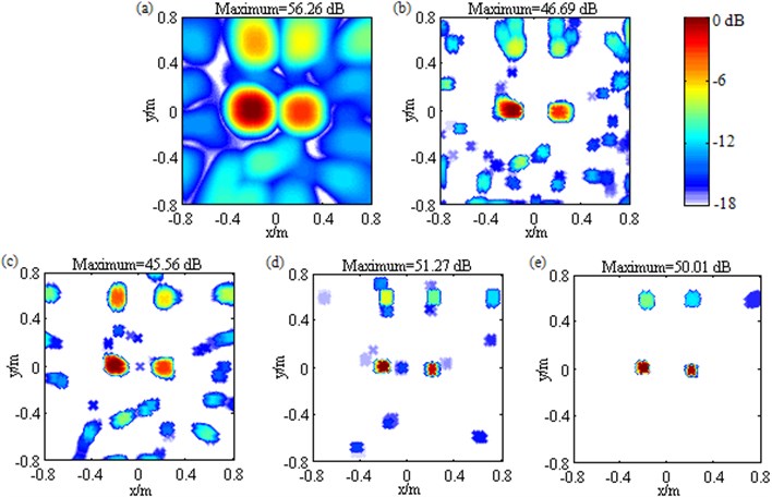
Similarly, Fig. 14 also displays the contour maps at 3000 Hz for the measurement with all the four loudspeakers simultaneously excited. The difference from Fig. 13 is that here pressure contributions of these loudspeaker sources are conspicuously unequal. As manifested by Fig. 14(a), they are 56.26 dB, 53.11 dB, 50.97 dB and 49.28 dB in turn, with a maximum gap of 7 dB. Fig. 14 presents similar phenomena with Fig. 13, indicating that Fourier-based deconvolution beamforming with the unconventional irregular 2D focus point distribution and the sidelobe suppression approach shown by Fig. 14(e) is optimal. In Fig. 14(e), mainlobes are narrowed remarkably, each mainlobe peak is created at a true loudspeaker location, being 56.72 dB, 53.44 dB, 50.79 dB and 48.89 dB, the calculated pressure contributions deviate from DAS’s results only by 0.46 dB, 0.33 dB, 0.18 dB and 0.39 dB in turn, and only one sidelobe with a maximum level of –16.07 dB appear. Consequently, the unconventional irregular 2D focus point distribution and the sidelobe suppression approach also can enhance the identification of these practical multiple sources with conspicuously unequal pressure contributions. The experimental conclusions demonstrated by Fig. 13-14 are in line with the simulation ones demonstrated by Figs. 5 and 6, proving that the conclusions are correct and the suggested approaches are effective in these practical multiple sources identification.
Moreover, corresponding to Fig. 7, Fig. 15 displays the contour maps at 1500 Hz under the condition that all the four loudspeakers are simultaneously excited. In Fig. 15(a), due to DAS’s poor-spatial-resolution and low-level-sidelobe characteristics at low frequencies, four mainlobes fuse mutually and the sidelobes are no higher than –12.14 dB in spite of their large coverage. In Fig. 15(b), Fourier-based NNLS deconvolution with only the conventional regular 2D focus point distribution fails for the loudspeaker sources at (–0.2, 0.6, 1) m and (0.2, 0.6, 1) m.
Fig. 14Contour maps showing identification results of multiple loudspeaker sources at 3000 Hz after different post-processing techniques: a) DAS; b) Fourier-based NNLS deconvolution with only the conventional regular 2D focus point distribution; c) Fourier-based NNLS deconvolution with only the unconventional irregular 2D focus point distribution; d) Fourier-based NNLS deconvolution with the conventional regular 2D focus point distribution and the sidelobe suppression approach; e) Fourier-based NNLS deconvolution with the unconventional irregular 2D focus point distribution and the sidelobe suppression approach. The sources have conspicuously unequal pressure contributions
In Fig. 15(c), four completely separated mainlobes are generated, each mainlobe peak is created at a true loudspeaker location, the pressure contributions are calculated as 52.77 dB, 52.60 dB, 51.66 dB and 52.40 dB that deviate from DAS’s results by only 0.46 dB, 0.32 dB, 0.15 dB and 0.19 dB in turn, only four sidelobes appear, and the MSL is as low as –13.18 dB, demonstrating that only with the unconventional irregular 2D focus point distribution, Fourier-based NNLS deconvolution can not only locate and quantify all the loudspeaker sources successfully but also obtain excellent spatial resolution and clean maps. In Fig. 15(d) and Fig. 15(e), totally confusing results come out. All these phenomena are in line with the ones shown in Fig. 7, proving the simulation conclusions that the incorporation of the sidelobe suppression approach will result in confusion when the mainlobes generated by DAS fuse with each other, and only with the unconventional irregular 2D focus point distribution, Fourier-based deconvolution beamforming is capable of working excellently in terms of source location, source quantification, spatial resolution amelioration and sidelobe removal at low frequencies are correct.
Fig. 15Contour maps showing identification results of multiple loudspeaker sources at 1500 Hz after different post-processing techniques: a) DAS;(b) Fourier-based NNLS deconvolution with only the conventional regular 2D focus point distribution; c) Fourier-based NNLS deconvolution with only the unconventional irregular 2D focus point distribution; d) Fourier-based NNLS deconvolution with the conventional regular 2D focus point distribution and the sidelobe suppression approach; e) Fourier-based NNLS deconvolution with the unconventional irregular 2D focus point distribution and the sidelobe suppression approach
6. Conclusions
When identifying sources in a relatively large region that is defined by a conventional regular focus point distribution, Fourier-based deconvolution beamforming would suffer from two obvious limitations: (1) significantly deteriorative location and quantification accuracy for sources away from the center of the focus region; (2) pronounced sidelobe contaminations. This paper focuses on remedying these limitations for 2D acoustic source identification. Our study has been motivated to provide the feasibility of using Fourier-based deconvolution beamforming to accurately and efficiently identify acoustic sources in a relatively large 2D region.
Two approaches are suggested. One is the novel focus point generation approach, the other one is the sidelobe suppression approach. The former can generate unconventional irregular 2D focus point distributions tending to make PSF more shift-invariant. The latter works by introducing a parameter positively associated with the number of iteration, computing a threshold as the largest component in the resulting vector minus the parameter and setting all components below the threshold to zero in each deconvolution iteration. Their effects are examined both with computer simulations and experimentally.
Some interesting conclusions have been drawn from our study: (1) replacement of the conventional regular focus point distribution with the unconventional irregular one is capable of remedying the first limitation successfully, but fails for the second one. (2) Combination of the unconventional irregular focus point distribution and the sidelobe suppression approach is capable of remedying both of the limitations resoundingly, when identifying a single source or multiple sources with unfused mainlobes. The mainlobe refers in particular to the one from traditional beamforming. (3) The sidelobe suppression approach is inadvisable when identifying multiple sources with mutually fused mainlobes. (4) The appropriate value range of the upper limit on the introduced parameter in the sidelobe suppression approach is 32 dB to 35 dB at each frequency. (5) Applications of these approaches barely sacrifice the original efficiency superiority.
References
-
Ginn K. B., Haddad K. Noise source identification techniques: simple to advanced applications. Proceedings of the Acoustics, Nantes, France, 2012, p. 1781-1786.
-
Cigada A., Ripamonti F., Vanali M. The delay and sum algorithm applied to microphone array measurements: numerical analysis and experimental validation. Mechanical Systems and Signal Processing, Vol. 21, Issue 6, 2007, p. 2645-2664.
-
Yardibi T., Bahr C., Zawodny N., Liu F., Cattafesta III L.N., Li J. Uncertainty analysis of the standard delay-and-sum beamformer and array calibration. Journal of Sound and Vibration, Vol. 329, Issue 13, 2010, p. 2654-2682.
-
Ramachandran R. C., Raman G., Dougherty R. P. Wind turbine noise measurement using a compact microphone array with advanced deconvolution algorithms. Journal of Sound and Vibration, Vol. 333, Issue 14, 2014, p. 3058-3080.
-
Brooks T. F., Humphreys W. M. A deconvolution approach for the mapping of acoustic sources (DAMAS) determined from phased microphone arrays. Journal of Sound and Vibration, Vol. 294, Issue 4, 2006, p. 856-879.
-
Brooks T. F., Humphreys W. M., Plassman G. E. DAMAS processing for a phased array study in the NASA Langley jet noise laboratory. 16th AIAA/CEAS Aeroacoustics Conference, Stockholm, Sweden, 2010.
-
Ehrenfried K., Koop L. Comparison of iterative deconvolution algorithms for the mapping of acoustic sources. AIAA Journal, Vol. 45, Issue 7, 2007, p. 1584-1595.
-
Richardson W. H. Bayesian-based iterative method of image restoration. Journal of the Optical Society of America, Vol. 62, Issue 1, 1972, p. 55-59.
-
Lucy L. B. An iterative technique for the rectification of observed distributions. Astronomical Journal, Vol. 79, Issue 6, 1974, p. 745-754.
-
Papamoschou D., Dadvar A. Localization of multiple types of jet noise sources. 12th AIAA/CEAS Aeroacoustics Conference, Cambridge, Massachusetts, USA, 2006.
-
Pascal J. C., Li J. F. Resolution improvement of data-independent beamformers. 36th International Congress and Exposition on Noise Control Engineering, Istanbul, Turkey, 2007, p. 4410-4419.
-
Yardibi T., Li J., Stoica P., Cattafesta III L. N. Sparsity constrained deconvolution approaches for acoustic source mapping. Journal of the Acoustical Society of America, Vol. 123, Issue 5, 2008, p. 2631-2642.
-
Dougherty R. P. Extensions of DAMAS and benefits and limitations of deconvolution in beamforming. 11th AIAA/CEAS Aeroacoustics Conference, Monterey, USA, 2005.
-
Hald J., Ishii Y., Ishii T., Oinuma H., Nagai K., Yokokawa Y., Yamamoto K. High-resolution fly-over beamforming using a small practical array. 18th AIAA/CEAS Aeroacoustics Conference, Colorado Springs, USA, 2012.
-
Yang Y., Ni J. M., Chu Z. G. Engine noise source identification based on DAMAS2 beamforming. Chinese Internal Combustion Engine Engineering, Vol. 35, Issue 2, 2014, p. 59-65.
-
Chu Z. G., Yang Y. Noise source identification for an engine based on FFT-non-negative least square (NNLS) deconvolution beamforming. Journal of Vibration and Shock, Vol. 32, Issue 23, 2013, p. 75-81.
-
Tiana-Roig E., Jacobsen F. Deconvolution for the localization of sound sources using a circular microphone array. Journal of the Acoustical Society of America, Vol. 134, Issue 3, 2013, p. 2078-2089.
-
Chu Z. G., Yang Y. Comparison of deconvolution methods for the visualization of acoustic sources based on cross-spectral imaging function beamforming. Mechanical Systems and Signal Processing, Vol. 48, Issues 1-2, 2014, p. 404-422.
-
Suzuki T. DAMAS2 using a point-spread function weakly varying in space. AIAA Journal, Vol. 48, Issue 9, 2010, p. 2165-2169.
-
Xenaki A., Jacobsen F., Tiana-Roig E., Fernandez-Grande E. Improving the resolution of beamforming measurements on wind turbines. Proceedings of 20th International Congress on Acoustics, Sydney, Australia, 2010, p. 2760-2767.
-
Xenaki A., Jacobsen F., Fernandez-Grande E. Improving the resolution of three-dimensional acoustic imaging with planar phased arrays. Journal of Sound and Vibration, Vol. 331, Issue 8, 2012, p. 1939-1950.
-
Christensen J. J., Hald J. Improvements of cross spectral beamforming. 32nd International Congress and Exposition on Noise Control Engineering, Seogwipo, Korea, 2003, p. 2652-2659.
Cited by
About this article

This work was funded by Chongqing Significant Application and Development Planning Project (No. cstc2015yykfc60003), Project of Chongqing Industry Polytechnic College (No. GZY201506-ZK) and National Natural Science Foundation of China (No. 51275540, 51275542).
