Sound field separation technique using the principle of double layer patch acoustic radiation modes

Liang, Guo; Haichao, Zhu; Rongfu, Mao; Junbo, Su; Changwei, Su

doi:10.21595/jve.2016.16929

Journal of Vibroengineering

Browse Journal

Submit article

Published: 31 March 2016

Check for updates

Sound field separation technique using the principle of double layer patch acoustic radiation modes

Guo Liang¹

Zhu Haichao²

Mao Rongfu³

Su Junbo⁴

Su Changwei⁵

^{1, 2, 3, 4, 5}National Key Laboratory on Ship Vibration and Noise, Naval University of Engineering, Wuhan, People’s Republic of China

Corresponding Author:

Zhu Haichao

Cite the article Download PDF

Downloads 1426

CrossRef Citations 1

Abstract

In order to solve the problems of near-field acoustic holography in applications such as external interference and aperture effects, a sound field separation technique using the principle of double layer patch acoustic radiation modes is proposed in this paper. The radiated acoustic pressures over two planar surfaces at certain distances from the sources are calculated first. Then, the effects resulting from the backscattering interference in non-free sound fields can be eliminated by a double-layer sound field separation technique. Next, data interpolation and extrapolation are performed on the separated data to increase the sound source's pressures on the holographic plane equivalently for holographic images with higher spatial resolution. Simulation and experimental results demonstrate that good agreements can be obtained with few measuring points.

1. Introduction

Near-field acoustic holography (NAH) [1] as a new technique in source identification has been used to reconstruct and visualize the complete radiated sound field. Specifically, ideal NAH requires an anechoic room, and the sound sources should be located on the same side of the measurement plane. However, most testing sites in practical applications cannot meet these requirements, and thus sound field separation techniques are introduced for eliminating the effects of interference sources [2]. Additionally, when NAH technique is applied, the holographic aperture should be greater than the actual size of the sound source in order to suppress the aperture effect. As complicated structures over large areas are analyzed, the number of measuring points should be increased, which significantly increases the workload and time requirements.

For solving the aforementioned problems, many advances have been made, such as the sound field separation method in noisy environments. The spatial Fourier transform method, which was used to separate incident and scattered fields has been proposed by Hallman and Bolton [3]. Statistically optimized NAH for sound field reconstruction in non-free-field environments with double layer pressure measurements [4], double layer velocity transducer array [5], and an array of pressure-velocity probes [6] can also be used. Further, the boundary element method (BEM) based on double-layer and single-plane measurements [7, 8] and the equivalent source method (ESM) using double-layer pressure measurements and particle velocity measurements [9-11] have been proposed for the same purpose. Recently, taking into account the scattering effect of disturbing sources, sound field separation methods based on single-plane and double-layer pressure measurements by using spherical wave superposition method were proposed [12, 13]. Based on the plane wave approximation and sound pressure superposition principles, a sound-field separation method for double arrays was also developed [14].

Aiming at solving the problems induced by aperture effects, data interpolation and extrapolation methods based on Patch NAH have been proposed. A data interpolation method based on the reconstruction of band-limited signals and data extrapolated by constructing the weighted normalization in the frequency domain was used by Xu et al. [15, 16]. A local NAH technique based on the equivalent source method and a distributed source-boundary point method were developed by Bi et al. [17, 18]. Moreover, a method based on wave-superposition-based method was proposed for enhancing the spatial resolution of NAH images [19, 20] and a NAH resolution enhancement method by using the interpolation of orthogonal spherical waves were studied [21, 22]. Methods for reducing the measuring points of holographic planes based on support vector regression (SVR) were also proposed by Mao, Du, et al. [23, 24].

However, these methods only focus on a single issue and lack comprehensive considerations to address multiple issues. When two issues exist simultaneously, we should combine the sound field separation technique with the Patch method based on data interpolation and extrapolation, and perform the optimization selection and control on the related parameters uniformly. Therefore, the disturbance of the interference source can be accurately eliminated by using fewer measurement data points, and the spatial resolution of the holographic plane can be further enhanced. Meanwhile, the workload in measurements can be significantly reduced. The combination of these two techniques will be of great theoretical value and significance when promoting the engineering application of NAH.

In the 1990s, Elliott, Borgiotti and Cunefare proposed an acoustic radiation mode analysis method that can serve as another approach for solving the acoustic radiation problems in low-to-medium frequency vibration structures [25-27]. Recently, Nie et al. [28] introduced a sound-field reconstruction formula for complex structures into the field of NAH based on acoustic radiation modes, and many favourable results were acquired in sound reconstruction and spatial resolution enhancement. In this paper, using sound radiation modes analysis and the reconstruction formula for sound fields, we consider the relationship between the relevant parameters and the proposed problems in a comprehensive account and propose a method to accurately eliminate the effects of interference sources, while simultaneously enhancing the spatial resolution of the holographic plane when fewer measuring points are used. Using the proposed method, the sound field distribution on the holographic plane with high spatial resolution can be obtained, which can provide accurate holographic data for further reconstruction of the sound field and have favourable engineering applicability.

2. Theory

2.1. Double-layer sound field separation technique

A vibration structure is placed in a homogeneous fluid whose sound velocity and density are $c_{0}$ and $ρ_{0}$ , respectively. The angular frequency of vibrations is $ω$ . By defining a structural surface $S_{o}$ , the whole space can be divided into inner space and outer space, respectively, denoted as $V_{i}$ and $V_{o}$ . The variable $n$ denotes the outer normal direction on the surface of the structure. In the outer space of the vibration structure, the pressure generated by the vibration follows the Helmholtz equation and satisfies the Neumann boundary conditions on the boundary surface. Moreover, the pressure satisfies the Sommerfeld radiation condition at infinite distance. From the Helmholtz integral equations for the inner space and outer space, the following relation is obtained:

1

\begin{array}{l} p_{o} (r^{'}), & (r' \in V_{o}), \\ p_{o} = p_{i}, & (r' \in S_{o}), \\ p_{i} (r^{'}), & (r' \in V_{i}), \end{array}\} = \iint_{S_{o}} [\frac{\partial p_{i} (r)}{\partial n} - \frac{\partial p_{o} (r)}{\partial n}] G (r | r') d S_{o},

where $r'$ and $r$ represent the position vectors on the measurement and vibration structure surface, respectively, and $G (r | r') = e^{j k |r' - r|} / 4 π |r' - r|$ denotes the free Green’s function. Based on acoustic radiation mode theory, the pressure matrix $P$ on the measurement plane can be obtained by:

2

P = G Φ C = Ψ C,

where $P = {[\begin{array}{l} p ({r'}_{1}) & p ({r'}_{2}) & \dots & p ({r'}_{M}) \end{array}]}^{T};$ the elements in the matrix $G$ are denoted as $G_{i j} = - j ρ_{0} ω s G (r_{i} | {r'}_{j})$ , $s$ denotes the element area after equal area partitioning on the structure surface, $C$ denotes the column vector of the expansion coefficients of different acoustic radiation modes, and $Ψ = G Φ$ denotes the mode matrix of the sound field distribution.

Fig. 1Illustration of the spatial arrangement of the target source, interference source and measurement planes. On the measurement plane S1, the pressure responses generated by the target and interference

Illustration of the spatial arrangement of the target source, interference source and measurement planes. On the measurement plane S1, the pressure responses generated by the target and interference

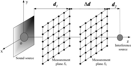
If the pressure is measured in two parallel planes, as displayed in Fig. 1, it can be expressed as in Eq. (2) in each plane. Considering that the pressure is a scalar quantity, we can obtain the following expression:

3

P_{1} = P_{1}^{1} + P_{2}^{1} = Ψ_{1}^{1} C_{1} + Ψ_{2}^{1} C_{2},

4

P_{2} = P_{1}^{2} + P_{2}^{2} = Ψ_{1}^{2} C_{1} + Ψ_{2}^{2} C_{2},

where the pressure responses on the holographic plane $S_{1}$ generated by the target source and the interference source are denoted as $P_{1}^{1}$ and $P_{2}^{1}$ , respectively and the pressure responses on the holographic plane $S_{2}$ generated by the target source and the interference source are denoted as $P_{1}^{2}$ and $P_{2}^{2}$ , respectively. $Ψ$ is the corresponding matrix of the sound distribution mode on the holographic plane generated by the source and $C$ is a the vector with expansion coefficients corresponding to the sound radiation modes of the target source and the interference source, $C_{1}$ and $C_{2}$ .

By combining Eq. (3) and Eq. (4), we can obtain:

5

C_{1} = (Ψ_{1}^{1} - Ψ_{2}^{1} (Ψ_{2}^{2})^{+} Ψ_{1}^{2})^{+} (P_{1} - Ψ_{2}^{1} (Ψ_{2}^{2})^{+} P_{2}),

6

C_{2} = (Ψ_{2}^{2} - Ψ_{1}^{2} (Ψ_{1}^{1})^{+} Ψ_{2}^{1})^{+} (P_{2} - Ψ_{1}^{2} (Ψ_{1}^{1})^{+} P_{1}),

where ‘+’ denotes the pseudo-inverse operation. When the condition number of $Ψ$ is comparatively large, regularization should be performed during the inversion process. Considering that the high-order radiation modes represent evanescent waves, the optimal order of the modes could be selected during the solution of the mode coefficient, so that the time consumption and workload in the calculation can be effectively reduced. The selection principle for the optimal order of the modes will be described in detail in the following sections.

By substituting Eq. (5) and Eq. (6) into Eq. (3) and Eq. (4), the pressure responses on the holographic plane $S_{1}$ generated by the target source and interference source can be expressed as:

7

P_{1}^{1} = Ψ_{1}^{1} * (Ψ_{1}^{1} - Ψ_{2}^{1} (Ψ_{2}^{2})^{+} Ψ_{1}^{2})^{+} (P_{1} - Ψ_{2}^{1} (Ψ_{2}^{2})^{+} P_{2}),

8

P_{1}^{2} = Ψ_{1}^{2} * (Ψ_{1}^{1} - Ψ_{2}^{1} (Ψ_{2}^{2})^{+} Ψ_{1}^{2})^{+} (P_{1} - Ψ_{2}^{1} (Ψ_{2}^{2})^{+} P_{2}) .

2.2. Patch technique based on data interpolation and extrapolation

As described in Eq. (2), the pressure generated by the sound source on the holographic plane is related to the field distribution modes of the sound source on the measurement plane, while the sound field distribution modes have a close relationship with the corresponding spatial positions. Fig. 2 displays the spatial distribution of the measurement plane $S_{1}$ and the holographic plane $S_{1}^{'}$ after data interpolation and extrapolation.

Fig. 2Illustration of data interpolation and extrapolation when using the Patch technique

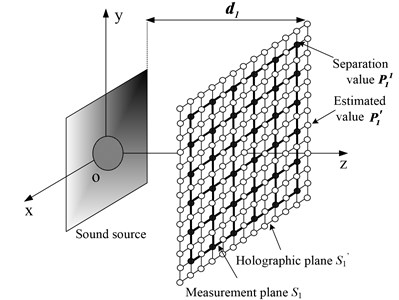
Based on the position information of all spatial points on the holographic plane $S_{1}^{'}$ , we can obtain the corresponding field distribution mode:

9

Ψ_{1}^{'} = G_{1}^{'} Φ_{1},

where $G_{1}^{'}$ denotes the transfer function matrix between the holographic plane $S_{1}^{'}$ and the target source plane, $Φ_{1}$ denotes the sound radiation modes on the target source surface. To obtain a cut-off of $Ψ_{1}^{'}$ with the same mode’s order and the expansion coefficient vector $C_{1}$ obtained in Eq. (5), the pressure matrix on the holographic plane $S_{1}^{'}$ containing more data can be estimated as:

10

P^{'} = Ψ_{1}^{'} C_{1} .

In order to retain the true value as much as possible and further reduce the estimation error, the pressure values in $P^{'}$ at the points whose spatial positions are identical to the measuring points are substituted by the values in $P_{1}^{1}$ , and finally, the holographic data $P_{r e c}$ for reconstructing the NAH sound field can be obtained.

To verify the sensibility of the errors of the proposed method, the error index, $E r r o r$ , can be defined as:

11

E r r o r = \frac{{‖P_{r e c} - P_{r e f}‖}_{2}}{{‖P_{r e f}‖}_{2}} \times 100 %,

where ${‖•‖}_{2}$ denotes the matrix 2-norm. $P_{r e c}$ denotes the pressure response generated by the target source after the two processing steps, and $P_{r e f}$ denotes the theoretical free field radiation radiated by the target source.

2.3. Selection of the optimal cut-off order of modes

Assuming that $P_{1 (M \times 1)}$ and $P_{2 (M \times 1)}$ denote the measurement data at $M$ measuring points on the measurement planes $S_{1}$ and $S_{2}$ , respectively, $Ψ_{(M \times N)}$ denotes the matrix of the sound field distribution modes corresponding to each source, and $C_{(N \times 1)}$ denotes the expansion coefficient vectors of sound radiation modes. Due to the matrix inversions are always ill-posed in the separation processes, some small measurement errors may be magnified to result a failure by the higher-order modes which are sensitive to errors. Therefore, there is no need to use all field distribution modes when performing sound field separation. In order to acquire a minimum separation error, the order of the sound field distribution modes, $Ψ_{(M \times N)}$ , should be cut off, and only the first $J$ -order modes $Ψ_{(M \times J)}$ are needed for further calculation. Based on the Helmholtz equation least squares method [29], the following steps are conducted in order to determine the optimal cut-off order.

First, the sound field distribution modes are cut off, with a cut-off order equal to 1, i.e., $J =$ 1. Then, the obtained cut-off field-distribution modes denoted as $Ψ_{(M \times J)}$ are substituted into Eq. (5) and Eq. (6) to solve the expansion coefficients of the first $J$ order field distribution modes, $C_{1 (J \times 1)}$ and $C_{2 (J \times 1)}$ . Next, the corresponding reconstructed pressure $P_{1 r e f}$ on the measurement plane $S_{1}$ is reconstructed in Eq. (3) to calculate the relative error between the reconstructed value $P_{1 r e f}$ and the measurement data $P_{1}$ by using the following ${‖L‖}^{2}$ -norm method:

12

{‖L‖}^{2} = \sum_{i = 1}^{M} {|P_{1 r e f} (r_{i}^{'}) - P_{1} (r_{i}^{'})|}^{2} .

Subsequently, the cut-off order of modes are increased one by one, i.e., $J = J + 1$ . By repeating the steps described above, the expansion coefficients with $J + 1$ order $C_{1 (J \times 1)}$ and $C_{2 (J \times 1)}$ are calculated again. Moreover, the relative error between the results on the reconstructed plane and the measurement plane can be calculated.

Finally, through the traversal on the cut-off order of modes $J$ , from 1 to $N$ , a set of relative errors which are correlated with $J$ could be obtained. The cut-off order corresponding to the minimum relative error was thus regarded as the optimal cut-off order $J_{o p}$ . It should be noted that the calculated $J_{o p}$ may be different given different numbers of measuring points at different frequencies. Generally, the higher the frequency value is, the larger the cut-off order $J_{o p}$ is.

3. Numerical simulation

3.1. Construction of the model

To verify the effectiveness and accuracy of the proposed method, two rigid pulsating spheres as the target source and interference source have been adopted for numerical simulations. The centre of the rigid pulsating sphere as the target source was located at the origin of coordinates, whose radius and vibration velocity were 0.1 m and 0.08 m/s, respectively. The radius and vibration velocity of another rigid pulsating sphere located at (0, 0, 0.85 m) were 0.15 m and 0.15 m/s, respectively. The two measurement planes, $S_{1}$ and $S_{2},$ have identical sizes (0.5 m×0.5 m), on which 64 measuring points (8×8) were distributed, centres of which were (0, 0, 0.2 m) and (0, 0, 0.35 m), respectively. In numerical calculations, the sound was transmitted through the air, and its velocity was set to 343 m/s. The theoretical values of the measurement planes were calculated according to the radiation induced by a rigid pulsating sphere [30]. In order to obtain simulation results closer to the actual measurements, a random white noise with an intensity of 30 dB was added to the simulated an actual measurement.

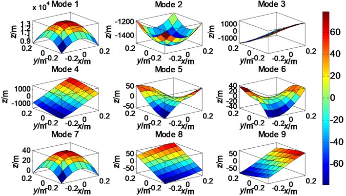
When processing the data collected on measurement planes using the proposed method, we first calculated the sound-field distribution modes of two rigid pulsating spheres. As stated above, the sound radiation modes are different at different frequencies. In the present work, $k a$ was set to 0.5, which means the frequency was set to 272.95 Hz. Using the target source as an example, the first nine-order sound radiation modes and the first nine field distribution modes on the measurement plane $S_{1}$ were calculated, with the results displayed in Fig. 3 and Fig. 4, respectively.

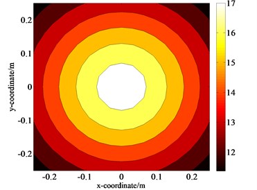
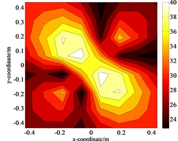
As described above, $k a =$ 0.5. Subsequently, the data on the measurement plane $S_{1}$ were calculated. Fig. 5(a) displays the amplitudes of pressure $p_{1}$ at the 64 measuring points (8×8). Then the pressure response $p_{1}^{1}$ generated by the target source was separated by using the proposed double-layer field separation technique, as displayed in Fig. 5(b). For comparison, the theoretical values of size 8×8 corresponding to the holographic data $p_{1}^{1}$ were calculated, as displayed in Fig. 5(c). Two-fold data interpolation and extrapolation were then conducted on $p_{1}^{1}$ to obtain the holographic data of size 17×17, in which the pressure values at the points whose spatial positions identical to the measuring point were substituted by the data $p_{1}^{1}$ , with the amplitudes displayed in Fig. 5(d). For further comparison, theoretical data of size 17×17 without interference was calculated, as displayed in Fig. 5(e).

Fig. 3The first nine-order sound radiation modes of the rigid pulsating sphere

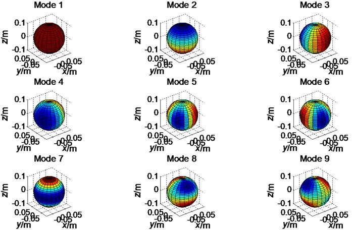
Fig. 4The first nine-order field distribution modes on the measurement plane S1

3.2. Analysis of the results

The comparative analysis between Fig. 5(a), (b) and (c) indicate that, when the interference source exists, a larger deviation occurs in high-pressure regions on the measurement plane, and dislocation appears in the regions with high and low pressures. Moreover, several regions with pseudo pressure appear, leading to great losses of image details. According to Eq. (11), the calculated measurement error compared with the theoretical value is approximately 52.23 %. After the two proposed steps, the results in the high-pressure regions returns to normal, and the pseudo pressure regions can be eliminated. The separation error with respect to the theoretical values for 8×8 measuring points is also calculated in Eq. (11) and reduced to only 0.86 % which means that the disturbance of the interference source can be effectively eliminated.

Fig. 5Distributions of the pressure amplitudes on the measurement plane S1 when ka= 0.5

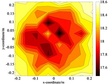
a) Initial data of size 8×8

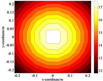
b) Separated data of size 8×8

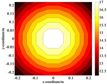
c) Theoretical data of size 8×8

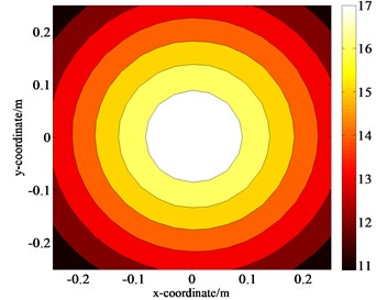
d) Processed data of size 17×17

e) Theoretical data of size 17×17

As shown in Fig. 5(b), (d) and (e), after two-fold data interpolation and extrapolation, the gradually-varied regions in the image become smoother. The sound field in the high-sound-pressure regions appears to be closer to the actual sound field generated by the rigid pulsating sphere, and some details in the images emerge. There is little difference between the holographic image and the theoretical image without interference and a favourable match between the estimated values and the separated values can be observed. According to Eq. (11), the error between the calculated pressure amplitudes in Fig. 5(d) and in Fig. 5(e) is only 0.89 %.

Conclusively, from the results at the 64 measuring points (8×8) as shown in Fig. 5(a), 289 holographic points (17×17) can be obtained, as shown in Fig. 5(d). By using the proposed method, we can not only eliminate the image distortion induced by the interference source but also accurately estimate the lost sound field information caused by fewer measuring points. In actual applications, the sound field information, which should be measured using 289 measuring points (17×17), can now be measured using 64 measuring points (8×8). This means that the workload due to the measurements is reduced by 77.85 %, which further proves the superiority of the proposed method described in this article.

3.3. Applicability research

In order to further verify the universal applicability of the proposed method, the relative separation and Patch errors for different values of $k a$ (from 0.1 to 3) which means the frequency was traversed within the range from 54.6 Hz to 1637.7 Hz were calculated. Fig. 6 shows the relationship between the relative errors and $k a$ . The relative errors are always below 3.0 %, which demonstrates that the processed field can be used to replace the free radiation field since the influence of the disturbing effect can be neglected at these frequencies.

Fig. 6Variation of errors as a function of ka

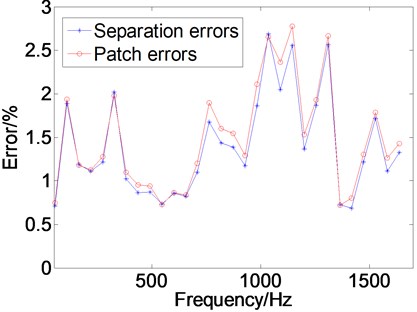
Fig. 7Correlated errors with variation of the SNR

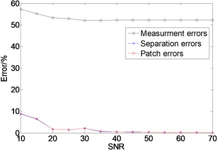
As the pressure data on the measurement planes are interfered by random white noise to obtain simulation results closer to the actual measurements. Different results will be obtained with the variation of the signal-to-noise ratio (SNR). Fig. 7 shows the relative errors with the variation of the SNR. It can be found that the relative errors between the theoretical free-field pressure and measurement data are larger than the separation and Patch errors. As shown in Fig. 7, the relative errors increased to 8 % at lower SNR, while the errors decreased slightly as the SNR increased, even below 1 %. These results again demonstrates that the interference pressure and the free-field radiated pressure can be separated effectively, and the interpolated and extrapolated data show good agreement with their matching theoretical values.

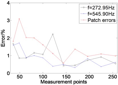
When the frequency fluctuates across a wide range, satisfactory results can be obtained when the number of measuring points is selected between 36 and 196. Fig. 8 shows the separation errors with different numbers of measuring points. If a conventional separation method requires 9×9 points, 6×6 measuring points can be used to obtain the same results by using the proposed method, which means a saving of 40 % workload and time measurement cost.

Fig. 8The separation errors with different numbers of measuring points

To further verify the generality of the proposed method, we also calculated the conditions when different kinds of sound sources were located on the two sides of the measurement planes. The target source was a 0.5 m×0.5 m rectangular panel, 0.008 m thickness, 7800 kg/m³ density, 2×10¹¹ Pa Young modulus, 0.28 Poisson’s ratio and centred at the origin of coordinates. The panel was driven at the position (0.125 m, 0.125 m, 0) by a point force of amplitude 10 N. Its radiation was calculated with a numerical approximation to Rayleigh’s integral. The interference source was a rigid pulsating sphere placed at (0, 0, 0.12 m), 0.05 m radius and 0.08 m/s vibration velocity. The sound pressure was measured at 8×8 points in two measurement planes of identical dimensions 1 m×1 m with a distance of 0.05 m between them. The two measurement planes were 0.04 m and 0.09 m from the plate. As the panel mainly vibrates with an order of (2, 2) at a modal frequency 612 Hz and the vibration amplitude of the panel was the largest, 600 Hz was selected as the excitation frequency for obvious results. A random white noise with an intensity of 30 dB was added to the measured pressure on each measurement surface to simulate an actual measurement.

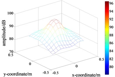
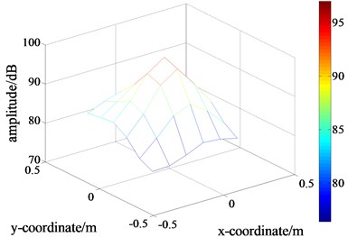
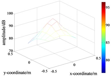
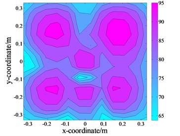
Fig. 9(a) shows the amplitudes of the measurement data of size 8×8 on the holographic plane $S_{1}$ . After the proposed separation step, the pressure responses generated by the target source independently on the measurement plane $S_{1}$ are displayed in Fig. 9(b). Fig. 9(c) compares the theoretical values of size 8×8 without the influence of the disturbing source. By performing the data interpolation and extrapolation step, holographic data of size 17×17 based on separated data of size 17×17 could be obtained, as depicted in Fig. 9(d). For comparison, theoretical data of size 17×17 without interference of the disturbing source was calculated, as displayed in Fig. 9(e).

As shown in Fig. 9, when the interference source exists, the high-sound-pressure regions obviously shift to greater peak values than the theoretical values, and the vibration mode of the panel presented in the holographic image approaches the (2, 2) mode. After processing the proposed two steps, the pressure distribution in the sound field can be accurately reconstructed, and the spatial resolution of the sound field can be effectively enhanced. According to Eq. (11) the separation error was calculated, and found to be 5.59 %. The results after performing the two-fold data interpolation and extrapolation on the separated data were compared to the theoretical values and the calculated Patch error was 6.46 %.

Fig. 9Distributions of the pressure amplitudes on the holographic plane S1 when ka= 0.55

a) Initial data of size 8×8

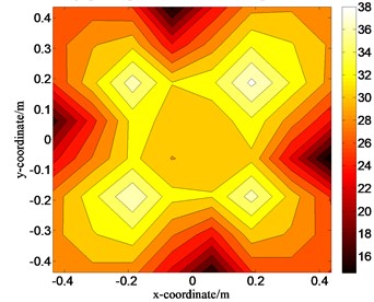
b) Separated data of size 8×8

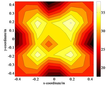
c) Theoretical data of size 8×8

d) Processed data of size 17×17

e) Theoretical data of size 17×17

4. Experiments

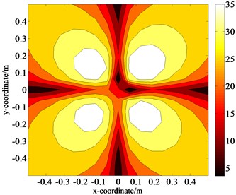
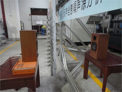
As shown in Fig. 10, the experiments were performed in an ordinary factory building. Two loudspeakers were then selected as sources for an in-depth study. The size of each loudspeaker was 0.23 m×0.14 m×0.13 m. One loudspeaker was adopted as the target sound source, centred as the origin of coordinates. The other loudspeaker driven coherently was used as disturbing source, placed opposite to the target source, at (0, –0.05 m, 0.6 m). The excitation signals of the two loudspeakers were generated by the same channel in the signal generator and then transmitted. The sound pressures were measured in a grid of 12×12 points with 0.05 m interspacing at the holographic planes $z_{1} =$ 0.1 m and $z_{2} =$ 0.3 m.

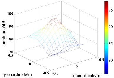
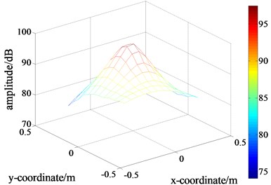
First, the loudspeaker as the target source was initiated, and the pressure distribution on the holographic plane $S_{1}$ was scanned and adopted as the theoretical value for further comparison, as displayed in Fig. 11(a). Subsequently, the two loudspeakers were turned on simultaneously and the sound pressure on two holographic planes, $S_{1}$ and $S_{2}$ , were acquired, as displayed in Fig. 11(b) and (c). By comparison, it can be observed that, due to the disturbance of the interference source, the pseudo-peaks appeared. The measurement errors were calculated to be 88.22 % and 95.78 %, respectively. Then, the data with a dimension of 6×6 were extracted and displayed in Fig. 11(e), (f) and (g), respectively.

Fig. 10A picture of the experiment set-up

By performing the proposed separation step, the pressure responses generated by the target source independently on the measurement plane $S_{1}$ were separated, displayed in Fig. 11(h). According to Eq. (11), the separation error between the sound-field separation results and the theoretical values using 6×6 measuring points was calculated as 11.22 %. Then, the processed results via data interpolation and extrapolation could be obtained, depicted in Fig. 11(b). The Patch error between the processed results and the theoretical values using 12×12 measuring points was calculated as 12.38 %. To verify the effectiveness of the experimental results, experiments at other frequencies were also conducted and the relative errors were listed in Table 1.

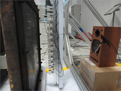
To further verify the proposed method, a boundary constraint steel plate with a size of 0.5 m×0.5 m and the thickness of 0.001 m was selected as the target source, and a loudspeaker with a size of 0.23 m×0.14 m×0.13 m was selected as the interference source, as shown in Fig. 12. The plate was set as the $X O Y$ coordinate plane and a rectangular coordinate system was constructed in which the interference source was located at (0, –0.05 m, 0.7 m). In total, 12 pressure sensors were included in the microphone array. The sound pressure was measured at 12×12 points in two measurement planes, $S_{1}$ and $S_{2}$ , with identical dimensions 0.66 m×0.66 m, located at (0, 0, 0.04 m) and (0, 0, 0.1 m), respectively. The excitation frequency was set to 292 Hz, the sampling frequency was set to 2048 Hz and the sampling time was 1 s. The complex pressure at each measuring point was calculated using the transfer function of a single reference source.

Table 1The relative errors at different frequencies

$f$ / Hz	Measurement error on the holographic plane using 36 measuring points (6×6)	Measurement error on the holographic plane using 36 measuring points (6×6)	Relative error between the results using the proposed method and the measured values using 144 measuring points (12×12)
240	86.42 %	84.75 %	12.38 %
380	102.68 %	70.88 %	14.63 %
480	124.28 %	94.55 %	14.95 %
580	85.89 %	110.37 %	15.64 %

Fig. 11Distributions of the sound pressure’s amplitude

a) The measured values on the holographic plane $S_{1}$ without interference

b) The measured values on the holographic plane $S_{1}$ with interference

c) The measured values on the holographic plane $S_{2}$ with the interference

d) The calculated values by performing the separation step

e) The extraction of the measured values on the holographic plane $S_{1}$ without interference

f) The extraction of the measured values on the holographic plane $S_{1}$ with interference

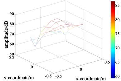
g) The extraction of the measured values on the holographic plane $S_{2}$ with interference

h) The calculated results using the proposed method

Fig. 12A picture of the experiment set-up

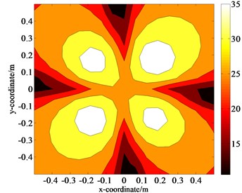
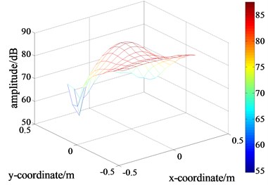
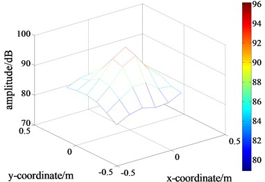
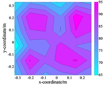
First, the plate was excited, and the pressure distribution on the holographic plane $S_{1}$ was scanned and extracted as the theoretical value for further comparison and analysis, as displayed in Fig. 13(f) and 13(a). Subsequently, the plate and loudspeaker were turned on simultaneously, and the pressure distributions on the two holographic planes, $S_{1}$ and $S_{2}$ , could be obtained. By comparison, due to the disturbance of the interference source, the errors are comparatively large, calculated as 60.16 % and 83.91 %, respectively. To verify the accuracy of the proposed technique, the data with a dimension of 6×6 points were then extracted from the pressure distributions on the two holographic planes, $S_{1}$ and $S_{2}$ , depicted in Fig. 13(b) and 13(c).

By performing the field separation step, the separated result was obtained, as displayed in Fig. 13(d). According to Eq. (11), the separated error was 12.75 %. Then, via data interpolation and extrapolation on the separated results, the Patch results were obtained, as displayed in Fig. 13(e). Compared with the theoretical values in Fig. 13(f), the processed results were quite close to the theoretical results, and the error was calculated to be only 10.24 %. The results indicated that the effects induced by the interference noise could be eliminated, and moreover, the spatial resolution of the holographic images could be effectively enhanced. On the other hand, 6 pressure sensors were sufficient to replace the 12 pressure sensors. The workload just be 6×6 $/$ (12×12) $=$ 0.25 $=$ 25 % of the actual workload, i.e., the workload and time consumption in the measurement could be significantly reduced.

5. Conclusions

To solve the problems of NAH in actual applications (such as the required free field and aperture effect), a double layer Patch NAH based on sound radiation modes was established. First, the mathematical relationship between the pressure on the measurement plane and the field distribution modes was derived. The effects of the interference sources were then eliminated using the double layer sound field separation technique. Then, the pressure values at more discrete points using data interpolation and extrapolation technique were estimated, which could provide more accurate holographic data for reconstructing the sound field. When performing the sound field separation and Patch step, the field distribution modes with the same order were selected and therefore, a uniform study and analysis of the relationship between the error and various parameters could be studied. With comprehensive consideration of the effects induced by the proposed method, the optimization selection and control on each parameter could be realized.

As indicated by the simulated and experimental results, the proposed method exhibits favourable universal applicability, and holographic data that are closer to the actual results using fewer measuring points were obtained, indicating that the processed technique is simple, economic and convenient for engineering applications.

Fig. 13Distributions of the pressure amplitude

a) The extraction of the measured values of size 6×6 without interference on $S_{1}$

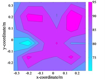
b) The extraction of the measured values of size 6×6 with interference on $S_{1}$

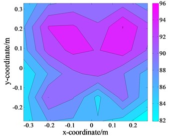
c) The extraction of the measured values of size 6×6 with interference on $S_{2}$

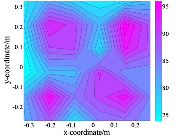
d) The separated values of size 6×6 on $S_{1}$

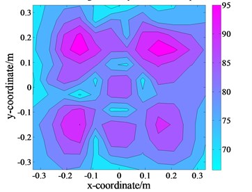
e) The processed results of size 12×12 using the double-layer sound field separation method on $S_{1}$

f) The measured values of size 12×12 without interference on $S_{1}$

References

Williams E. G. Fourier Acoustics: Sound Radiation and Nearfield Acoustical Holography. Academic Press, London, 1999.

Publisher
Wang R., Chen J., Jia W. Q., et al. Acoustic field separation technique with single holographic plane based on wave superposition algorithm and statistically optimal near field acoustical holograph. Journal of Vibration and Shock, Vol. 31, Issue 22, 2009, p. 112-117.

Search CrossRef
Hallman D. L., Bolton J. S. A technique for performing source identification in reflective environments by using nearfield acoustic holography. Proceedings of NoiseCon, Williamsburg, VA, 1993.

Search CrossRef
Jacobsen F., Chen X. Y., Jaud V. A comparison of statistically optimized near field acoustic holography using single layer pressure-velocity measurements and using double layer pressure measurements. The Journal of the Acoustical Society of America, Vol. 123, Issue 4, 2008, p. 1842-1845.

Publisher
Fernandez-Grande E., Jacobsen F. Sound field separation with a double layer velocity transducer array. The Journal of the Acoustical Society of America, Vol. 130, Issue 1, 2011, p. 5-8.

Publisher
Jacobsen F., Jaud V. Statistically optimized near field acoustic holography using an array of pressure-velocity probes. The Journal of the Acoustical Society of America, Vol. 121, Issue 3, 2007, p. 1550-1558.

Publisher
Langrenne C., Melon M., Garcia A. Boundary element method for the acoustic characterization of a machine in bounded noisy environment. The Journal of the Acoustical Society of America, Vol. 121, Issue 5, 2007, p. 2750-2757.

Publisher
Valdivia N. P., Williams E. G., Herdic P. C. Approximations of inverse boundary element methods with partial measurements of the pressure field. The Journal of the Acoustical Society of America, Vol. 123, Issue 1, 2008, p. 109-120.

Publisher
Bi C. X., Bolton J. S. An equivalent source technique for recovering the free sound field in a noise environment. The Journal of the Acoustical Society of America, Vol. 131, Issue 2, 2012, p. 1260-1270.

Publisher
Bi C. X., Chen X. Z., Chen J. Sound field separation technique based on equivalent source method and its application in nearfield acoustic holography. The Journal of the Acoustical Society of America, Vol. 123, Issue 3, 2008, p. 1472-1478.

Publisher
Bi C. X., Hu D. Y., Zhang Y. B., et al. Reconstruction of the free-field radiation from a vibrating structure based on measurements in a noisy environment. The Journal of the Acoustical Society of America, Vol. 134, Issue 4, 2013, p. 2823-2832.

Publisher
Song Y. L., Lu H. C., Jin J. M. Sound wave separation method based on spatial signals resampling with single layer microphone array. Acta Physica Sinica, Vol. 63, Issue 19, 2014, p. 195-204.

Publisher
Bi C. X., Hu D. Y., Xu L., et al. Recovery of the free field in a noisy environment by using the spherical wave superposition method. Acta Acustica, Vol. 39, Issue 3, 2014, p. 339-346.

Search CrossRef
Li Y. Z., Zhang Y. B., Bi C. X. An investigation of beamforming using a double layer array. Journal of Hefei University of Technology, Vol. 35, Issue 8, 2012, p. 1049-1053.

Search CrossRef
Xu L., Bi C. X., Chen X. Z., et al. Resolution enhancement of near-field acoustic holography based on Papoulis-Gerchberg algorithm. Chinese Science Bulletin, Vol. 53, Issue 14, 2008, p. 1632-1639.

Publisher
Xu L., Bi C. X., Wang H., et al. Hologram pressure field weighted norm extrapolation method. Acta Physica Sinica, Vol. 60, Issue 11, 2011, p. 406-416.

Publisher
Bi C. X., Chen X. Z., Xu L., et al. Patch nearfield acoustic holography based on the equivalent source method. Science in China (Series E: Technological Sciences), Vol. 37, Issue 9, 2007, p. 1205-1213.

Search CrossRef
Bi C. X., Yuan Y., He C. D., et al. Patch nearfield acoustic holography based on the distributed source boundary point method. Acta Physica Sinica, Vol. 59, Issue 12, 2010, p. 8646-8655.

Publisher
Zhang X. Z., Bi C. X., Xu L., et al. Resolution enhancement of nearfield acoustic holography by the wave superposition approach. Acta Physica Sinica, Vol. 59, Issue 8, 2010, p. 5564-5571.

Publisher
Xu L., Bi C. X., Chen J. Algorithm and experimental investigation of patch nearfield acoustic holography based on wave superposition approach. Acta Physica Sinica, Vol. 56, Issue 5, 2007, p. 2776-2783.

Publisher
Xu L., Chen X. Z., Bi C. X., et al. Nearfield acoustic holography resolution enhancing method based on interpolation using orthogonal spherical wave source. Journal of Zhejiang University (Engineering Science), Vol. 43, Issue 10, 2009, p. 1808-1811.

Search CrossRef
Xu L., Bi C. X., Chen X. Z., et al. Patch near-field acoustic holography by extrapolation using orthogonal spherical wave source. Journal of Mechanical Engineering, Vol. 46, Issue 4, 2010, p. 1-7.

Publisher
Mao R. F., Zhu H. C., Liu Z. Z., et al. Experimental study on reduction of measuring points number on hologram using support vector regression. Journal of Vibration and Shock, Vol. 29, Issue 3, 2010, p. 128-131.

Search CrossRef
Du X. H., Zhu H. C., Mao R. F., et al. Patch near-field acoustic holography based on support vector regression. Acta Acustica, Vol. 37, Issue 3, 2012, p. 286-293.

Search CrossRef
Elliott S. J. Radiation modes and the active control of sound power. The Journal of the Acoustical Society of America, Vol. 94, Issue 4, 1995, p. 2194-2204.

Publisher
Borgiotti G. V. The power radiated by a vibrating body in an acoustic fluid and its determination from boundary measurement. The Journal of the Acoustical Society of America, Vol. 88, Issue 4, 1990, p. 1884-1893.

Publisher
Cunefare K. A., Currey M. N. On the exterior acoustic radiation modes of structure. The Journal of the Acoustical Society of America, Vol. 96, Issue 4, 1994, p. 2302-2312.

Publisher
Nie Y. F., Zhu H. C. Acoustic field reconstruction using source strength density acoustic radiation modes. Acta Physica Sinica, Vol. 63, Issue 10, 2014, p. 256-267.

Publisher
Wu S. F. On reconstruction of acoustic pressure fields using the Helmholtz equation least squares method. The Journal of the Acoustical Society of America, Vol. 107, Issue 5, 2000, p. 2511-2522.

Publisher
Wang Z., Wu S. F. Helmholtz equation-least squares method for reconstructing the acoustic pressure field. The Journal of the Acoustical Society of America, Vol. 102, Issue 4, 1997, p. 2020-2032.

Publisher

Cited by

Reconstruction of Acoustic Radiation of a Vibrating Structure Located in a Half-Space Bounded by a Passive Surface with Finite Acoustic Impedance

Daren Zhou | Huancai Lu | D. Michael McFarland | Yongxiong Xiao

(2020)

About this article

Received

26 January 2016

Accepted

14 March 2016

Published

31 March 2016

SUBJECTS

Acoustics, noise control and engineering applications

DOI

https://doi.org/10.21595/jve.2016.16929

Keywords

sound field separation technique

double layer patch acoustic radiation modes

data interpolation and extrapolation

near-field acoustic holography

Acknowledgements

The authors would like to thank the referees for their review of this manuscript. The work is supported by the National Natural Science Foundation of China, Grant No. 51305452.

Author Contributions

Guo Liang made a major contribution to the research. Zhu Haichao made guidance work to the research. Mao Rongfu gave consultative opinions to the paper. Su Junbo and Su Changwei made simulation calculations to the paper.

This is an open access article distributed under the Creative Commons Attribution License, which permits unrestricted use, distribution, and reproduction in any medium, provided the original work is properly cited.