Numerical computation and optimization design of pantograph aerodynamic noise

1. Introduction

When the high-speed train is running quickly, a serious disturbance for air is generated due to its convex-concave parts, causing it to produce complex flow separation and a series of vortex shedding and breaking. Consequently, the strong pulsating pressure field of the external air is resulted in and converted into the aerodynamic noise [1-3]. Currently, the main aerodynamic noise sources of the high-speed train are identified by means of the acoustic analogy theory, low-noise wind tunnel and array technology [4-6]. As a prominent part on the roof of the high-speed train, the aerodynamic noise of the pantograph is increased significantly with the increases of the train speed. To control the pantograph aerodynamic noise, related research institutions in Japan have conducted a series of experiments and theoretical analysis and developed the pantograph fairing with a big length [7-9], achieving significant noise reduction effect. However, when the speed is more than 300 km/h, the air flow will be split by the pantograph fairing. And the continuously repeated vortex will be generated in the split area of the airflow, which enlarges the noise of the pantograph fairing [10]. Therefore, the researches on the aerodynamic noise of the pantograph are necessary.

Due to the complex characteristics of the flow field near the pantograph, it is difficult to be researched through theoretical analysis. Currently, the experimental method and numerical simulation are primarily applied for the researches on the pantograph aerodynamic noise of the high-speed train. In terms of experiments, the real train experiment and wind tunnel experiment are mainly included, but both have their deficiencies. Due to the influence of the external noise, the results of the real train experiment are difficult to be reliable. The high-speed train models are scaled down proportionally by most of wind tunnel experiment, which is quite different from the actual structure. However, the numerical simulation method can be carried out quickly and effectively and therefore are widely used. Limited by the computing resources and time, the current research work focuses on the pantograph aerodynamic characteristics under steady state, and the research model has also been greatly simplified [11].

Siano has numerically computed the pantograph aerodynamic noise and verified the accuracy of the numerical results by compared with that of the experiment [12]. Nevertheless, the actual situation cannot be reflected due to the oversimplification of the pantograph computation model. The aerodynamic noise of the pantograph insulators is computed and the optimization design of its shape is conducted by Xiao [13]. However, the aerodynamic characteristics of the insulator are only researched simply by him, while this structure is not applied to the pantograph in the research.

In this paper, by means of the switch inside the numerical model, the small-scale pulsation on the near wall is simulated by URANS method. Areas away from the wall are adjusted to the sub grid scale (SGS) models automatically, which is simulated for the vortex movement by LES method. Via the automatically adjustable method in accordance with local grids, not only the advantage concerning the small computation amount of URANS method can be shown in the boundary layer, but also the large-scale vortex movement can be simulated in the areas away from the wall. Based on the above method, firstly, the aerodynamic resistance and lift of the pantograph are computed, which is compared with the experimental results in order to verify the reliability of the numerical method. Next, the pantograph aerodynamic characteristics and sound field distribution are computed to optimize its aerodynamic noise.

2. Geometric modeling and grid generation

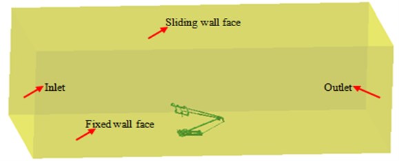
The pantograph geometric model applied in this paper is shown in Fig. 1, which is consisted of the pantograph head, push rod, base and other structures. According to the pantograph geometric model, its surface is extracted to divide into grids. As a result, the aerodynamic grid model of the pantograph can be obtained as Fig. 2, which has 3569 elements and 4285 nodes. Since the speed of the high-speed train is within the subsonic range, its control equation is the elliptic equation, and the whole flow field area is affected by the pressure wave. To reduce the impact of the computational domain size on the computational result, the computational domain used in this paper is selected as follows. The height $h$ from the pantograph base to the top of the pantograph head is chosen as the characteristic length, wherein, the inlet direction is taken as 8$h$, the outlet direction is 15$h$, the left and right sides are 4$h$, and the top is 8$h$. The model of the computational domain is shown in Fig. 3. During designing grids, the anisotropic grids required by RANS equation are applied on the near wall, while the isotropic unstructured grids are tried to be applied on the areas away from the wall. Finally, there are more than one million elements existing in the computational domain of the pantograph.

Fig. 1Pantograph geometric model

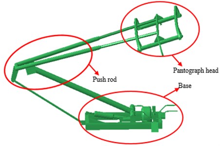
Fig. 2Aerodynamic grid model of the pantograph

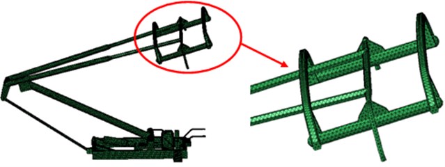
Fig. 3The computational domain of the pantograph

3. Numerical simulation of pantograph aerodynamic characteristics

As pantograph flow field has obvious unsteady characteristics, the unsteady computation is required for researching the unsteady aerodynamic characteristics of the pantograph. The computational method of the unsteady characteristics includes direct numerical simulation (DNS), large eddy simulation (LES) and unsteady Reynolds-averaged (URANS) methods. The grid quantity and the computing time required by DNS method are very enormous, which cannot be used for engineering computation. The medium and large-scale vortex structures of the flow field can be reflected better and the transient flow field information can be provided in detail by LES method, the grid quantity required by the computation is still large, especially in the vicinity of the near wall [14]. Despite the advantage of small computation amount, URANS method is difficult to simulate the flow of large separation and the unsteady complex flows accurately, such as the vibration and aerodynamic noise, etc. The advantages of DES method in combination with URANS method and LES method are attempted in the paper for the computation. By means of the switch inside the numerical model, the small-scale pulsation on the near wall is simulated through URANS method. Areas away from the wall are adjusted to the sub grid scale (SGS) models automatically, which are simulated for the vortex movement by LES method. Via the automatically adjustable method in accordance with local grids, not only the advantage concerning the small calculation amount of URANS method can be shown in the boundary layer, but also the large-scale vortex movement can be simulated in the areas away from the wall

At present, the commonly used DES methods [15] are based on SA turbulence model and SST equation, respectively. As shown in many researches [16, 17], the application of DES method in the flow field of the ground vehicles, the vortex structures of the aircraft wing trail, and the high attack angle of the aircraft can get better results. In the paper, DES method base on SST equation is applied, and N-S equation is selected as the control equation and the finite volume method is used in the discreteness of the equation. Roe format is used in the convection term for the discreteness, and the restriction function is added to improve the precision of the interpolation. Furthermore, the second-order center difference is adopted in the viscous term for the discreteness, and SGS method is used in the time term. The unsteadily computation time step is 0.0001 s, and the number of iteration step is 5. DES formula based on SST equation is as follow:

wherein, $\rho$ is the fluid density, $U_i$ is the average velocity component along the direction $i$, $k$ represents the turbulent kinetic energy of the turbulent motion, $P_k$ indicates the generation term of the turbulent kinetic energy, and $P_k={\tau }_{ij\partial }{U}_i/\partial x$, ${\tau }_{ij}$ is the Renault stress. $\omega$ is the turbulent dissipation rate, $\mu$ is the dynamic viscosity coefficient, ${\mu }_k$ represents the eddy viscosity, and ${\mu }_k=\rho k/\omega$. $F_1$ is the mixed function, which is 1 within the boundary layer and whose model is $k$-$\omega$ model, and which is converted to 0 in the regions away from the wall and whose model transfers to $k$-$\epsilon$ model. ${\beta }^{*}$, $\beta$, $\gamma$, ${\sigma }_k$ and ${\sigma }_{\omega }$ can all be expressed by $\phi$. If the factor in the original $k$-$\omega$ model is expressed by ${\phi }_1$ and the factor in $k$-$\epsilon$ model is represented by ${\phi }_2$, the constant $\phi$ of SST equation model can be expressed as follows:

wherein, all coefficients in $k$-$\omega$ model are ${\sigma }_{k1}=$ 0.85, ${\sigma }_{\omega 1}=$ 0.5, ${\beta }_1=$ 0.075, ${\beta }^{*}=$0.09, and ${\gamma }_1=$0.5532. After conversion, all coefficients in $k$-$\epsilon$ model are ${\sigma }_{k2}=$1.0, ${\sigma }_{\omega 2}=$ 0.856, ${\beta }_2=$0.0828, ${\beta }^{*}=$0.09, and ${\gamma }_1=$0.4404.

The basic idea of DES method based on SST equation is to remain $\omega$ Eq. (2) in SST equation unchanged and introduce the turbulence scale parameter $l_{k-\omega }$ into the dissipative item of equation $k$ Eq. (1). Therefore, the Eq. (1) has turned into the following form.

In the formula, $l_{k-\omega }=k^{0.5}/{\beta }^{*}\omega$. In DES method, $l_{k-\omega }$ is substituted by the scale parameter $\mathrm{m}\mathrm{i}\mathrm{n}\left(l_{k-\omega },C_{DES}∆\right)\text{,}$ wherein, $\mathrm{\Delta }$ is the maximum edge of the grid element, namely $\left(∆\right)=\mathrm{m}\mathrm{a}\mathrm{x}$($∆x,∆y,\mathrm{}∆z$). The constant $C_{DES}$ can be derived by $F_1$, $C_{DES}=\left(1-F_1\right)C_{DES}^{k-\epsilon }+F_1{C}_{DES}^{k-\omega }$, wherein, 0.61 and 0.78 are taken for $C_{DES}^{k-\epsilon }$ and $C_{DES}^{k-\omega }$, respectively [15].

After the above configuration, as $\omega$ value is quite large and $k$ value is finite in the boundary layer near wall, $l_{k-\omega }$ is much less than the scale of grid element, SST equation model plays a role, and Reynolds-averaged algorithm can be applied. In the areas away from the wall, $\omega$ value decreases, and when $l_{k-\omega }$ is greater than $C_{DES}∆$, the model is converted to SGS Reynolds stress model simulated by large eddy.

The computational boundary conditions are set as follows. The inlet is the boundary condition of the speed, and the inflow velocity is set to be 350 km/h. The outlet is the boundary condition of the pressure, whose outer field has applied the condition of the sliding wall. In addition, in order to simulate the real flow field characteristics and in consideration of the relative motion between the train and the ground, the condition of the mobile wall is applied on the ground, whose moving speed is same as the train speed.

4. Numerical computation of pantograph aerodynamic characteristics and noise

4.1. Numerical computation of pantograph aerodynamic characteristics

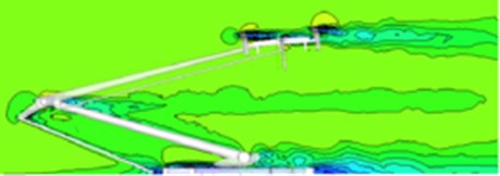
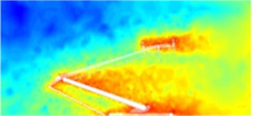
According to the above analysis, the pantograph computation model established in this paper is effective. Through this computational model, the speed distribution of the pantograph under the fluid can be computed, as shown in Fig. 4. It can be seen that the characteristics similar to the cylinder flow and rear-order station flow are formed by the pantograph when the fluid pass it. The higher velocity areas are mainly concentrated in the pantograph head, push rod and base part, and it is mainly because some protrusions existing in these places have some interference effect on the fluid flow.

Fig. 4Speed distribution contour of the pantograph

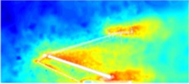
At the high speed, the lift and resistance of the pulsation are generated by the rear vortex shedding and breaking of the pantograph, thus producing some aerodynamic noise. The cycles of vortex strength, shedding and breaking are different due to different speeds of the train. As shown in Fig. 5, the biggest vorticity regions of the pantograph are appeared in the pantograph head, push rod and base. For the push rod, its big vorticity is caused by the complex turbulent flow formed by the close angles between the upper and lower push rods and the inlet directions, in combination with its smaller diameter push rod. There are many components in the pantograph head and base, therefore forming more disordered vortexes.

Fig. 5Vorticity distribution contour of the pantograph

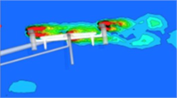
a) Pantograph head

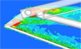
b) Push rod

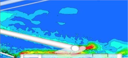
c) Base

4.2. Numerical computation of the pantograph aerodynamic noise

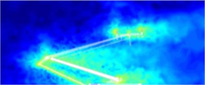
As seen from Fig. 5, the biggest vorticity regions are appeared in the pantograph head, push rod and base, and the effect of bigger vorticity on the sound field is necessary to be researched. Aerodynamic characteristics of the pantograph are computed by means of FLUENT software in the above analysis. Then, the result is imported into Virtual.lab software. The surface of the pantograph geometric model is extracted in Fig. 1, the boundary element meshes are divided, and the element length should be set based on the requirements of the computational frequency. Finally, the boundary element mesh model is obtained and shown in Fig. 6, with a total of 1265 elements and 1056 nodes. Then, the boundary element mesh model is also imported into Virtual.lab software. Next, elements and nodes of aerodynamic characteristics and boundary element model are renumbered to avoid conflict. Finally, aerodynamic characteristic results are mapped onto the boundary element model in order to achieve coupling between acoustic and structure. In this way, all features of the structural meshes will also be obtained by the boundary element meshes. As a result, acoustic characteristics of the pantograph can be computed numerically. Based on the above method, the distribution of sound source intensity for the pantograph is computed at 40 Hz, 140 Hz and 500 Hz as Fig. 7. It could be seen that the distribution of the sound source intensity is similar to that of the vorticity, with greatest values appeared in the pantograph head, push rod and base. In addition, the sound source intensity is decreased gradually in the pantograph head, push rod and base along with the increase of the frequency, which is caused by that the resonance effect between the pantograph and wind is majorly appeared within 100 Hz.

Fig. 6Boundary element model of the pantograph

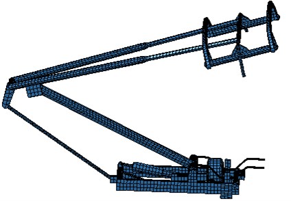
Fig. 7Distribution of sound source intensity for the pantograph

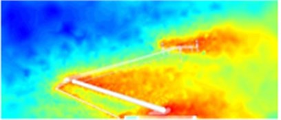
a) 40 Hz

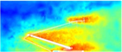
b) 140 Hz

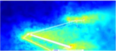
c) 500 Hz

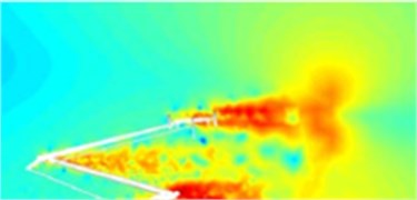
The sound pressure distribution of the pantograph under the fluid can be obtained by further processing the sound source intensity in Fig. 7, as shown in Fig. 8. As can be seen from Fig. 7 and Fig. 8, wherever the sound source intensity is greater, the pantograph sound field is also larger. Moreover, the distribution of the pantograph sound field has presented a decreasing trend with the increasing frequency.

Fig. 8Distribution of the pantograph sound field

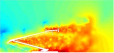
a) 40 Hz

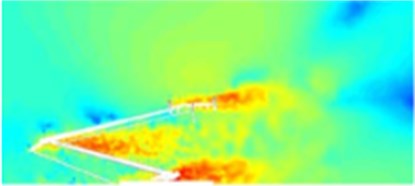
b) 140 Hz

c) 500 Hz

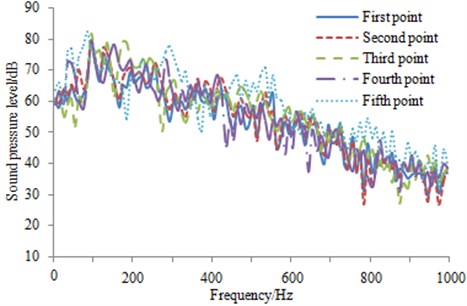
In order to observe the pantograph flow noise distribution under the effect of wind speed, five observation points are arranged right over the pantograph, on the center of the bottom, at front and rear positions, as well as in the 45° angle, as shown in Fig. 9. SPL at the observation points are extracted for comparison, as shown in Fig. 10. It could be seen that the corresponding SPL are reduced with the increasing frequency. In addition, the maximum SPL at the observation points are basically appeared within 100 Hz, which further verifies the above analysis.

Fig. 9Locations of the pantograph observational points

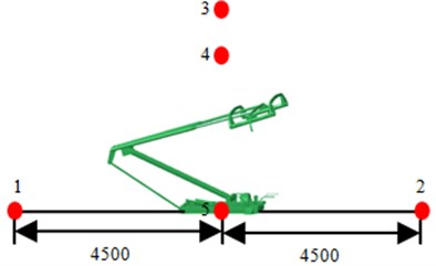
a) Side view

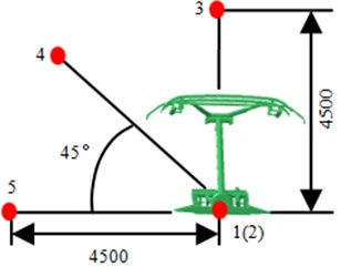
b) Front view

Fig. 10SPL comparison at the observational points

5. Experimental verification of pantograph aerodynamic characteristics

The pantograph is composed of many components, so its structure is quite complex. It is necessary to verify the aerodynamic model by experiments, otherwise the subsequent analysis can’t be ensured.

The experiments of pantograph are conducted in FD-09 low-speed wind tunnel [18]. By means of the installation of shrinking bottom plate in the wind tunnel experiment section, a new experimental section with the width of 3 m and height of 2 m is formed; whose maximum experimental wind speed can reach 380 km/h.

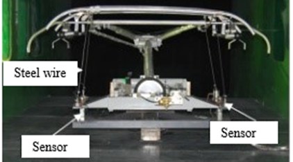
The overall aerodynamic force of the pantograph is measured by a six-component cassette strain scale and some sensors, with the aim to primarily measure the overall resistance and lift, as well as overall pantograph aerodynamic characteristics under different wind velocities ($V=$210 km/h-370 km/h). In the wind tunnel experiment section, an adapter seat is installed, which is stretched out of the shrinking floor to connect with the cassette scale. On the scale, a triangular adapter seat is linked as Fig. 11.

Fig. 11Pantograph test procedure

Through the above analysis, the pantograph aerodynamic lift and resistance are computed and compared with those of the experimental, as shown in Fig. 12. As can be seen from Fig. 12, the experimental and simulation results are consistent with each other, which indicates that the numerical computation model is reliable and can be used for the subsequent analysis.

Fig. 12Comparison of experimental and simulation results for pantograph aerodynamic resistance and lift

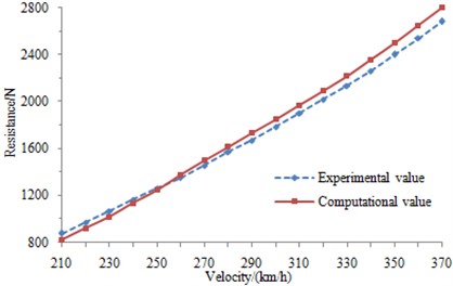
a) Comparison of experimental and simulation results for the aerodynamic resistance

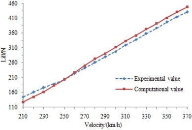
b) Comparison of experimental and simulation results for the aerodynamic lift

6. Numerical optimization of the pantograph aerodynamic noise

Pantograph aerodynamic noise is relatively large according to the above analysis, and therefore, it is necessary to be optimized. At present, the optimization of noise is mainly focused on two aspects, namely, improving the structure and applying sound absorption material. As the cost required for the structural improvement is high and there are many parts in the pantograph, its structural optimization is difficult to be conducted by a certain optimization algorithm. Therefore, the porous sound absorption material is selected to apply on the pantograph in this paper.

A layer of 3 mm-thick glass wool is applied on the cylindrical rod of the pantograph head and push rod. In addition, glass wool is also applied on base of the pantograph. The fluid medium in glass wool is air. The fluid density is 1.225 kg/m³. Sound speed in fluid is 340 m/s. Porosity rate is 0.99. Flow resistivity is 9000 rayl/m. The structural tortuosity is 1. Viscoelastic characteristic length is 1.92 e^-4m. Thermodynamic characteristic length is 3.84 e^-4m. Material density is 16 kg/m³. Young’s modulus is 1 e⁵, and Poisson’s ratio is 0.3.

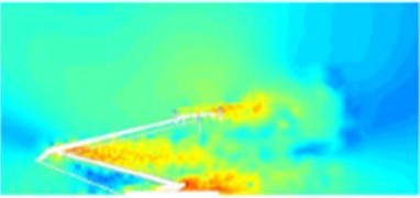
Based on the verified model, the distribution of sound source intensity is computed after applying sound absorption material, as shown in Fig. 13. From the comparison of Fig. 7 and Fig. 13, the sound source intensity on the pantograph head, push rod, and base has improved to some extent. This improvement is mainly formed because many holes existing inside the sound absorption material will prevent the sound appropriately and transfer it into the heat for dissipation. Moreover, the characteristic which sound source intensity reduced along with the increase of frequency is also remained.

Fig. 13Sound source intensity distribution after applying sound absorption material

a) 40 Hz

b) 140 Hz

c) 500 Hz

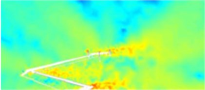
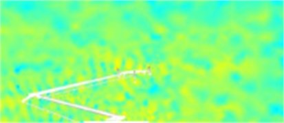
Fig. 14Sound field distribution after applying sound absorption material

a) 40 Hz

b) 140 Hz

c) 500 Hz

Based on sound source intensity distribution, the sound field distribution on the pantograph surface can be obtained as shown in Fig. 14. From the comparison of Fig. 13 and Fig. 14, wherever the sound source intensity is greater, the sound field is also larger. In addition, the sound field on the pantograph surface is improved relatively after applying sound absorption material, as seen from the comparison of Fig. 8 and Fig. 14. Moreover, the characteristic which sound field reduced along with the increase of frequency is also remained.

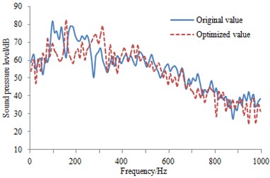
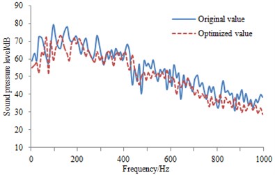
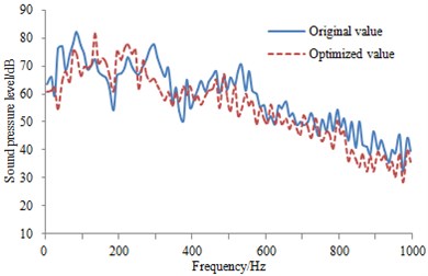
In order to further observe the improvement effect of the sound absorption material on the pantograph aerodynamic noise, SPL of the observational points in Fig. 9 are extracted and compared with the original result, as shown in Fig. 15. As can be seen from the figure, the most optimized peaks are reduced to a certain degree. Generally speaking, the aerodynamic noise is improved, and it showed that applying sound absorption material is reliable. In addition, this measure is easily realized and cost is also low.

Fig. 15SPL comparison at the observation points before and after the optimization

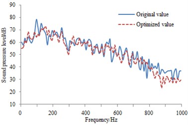
a) SPL comparison at the first observation point

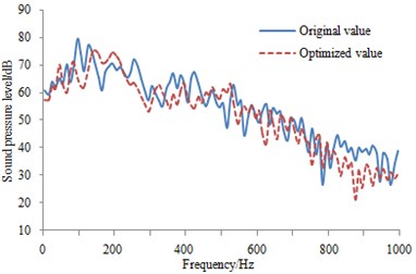
b) SPL comparison at the second observation point

c) SPL comparison at the third observation point

d) SPL comparison at the fourth observation point

e) SPL comparison at the fifth observation point

7. Conclusions

1) By means of the switch inside the numerical model, the small-scale pulsation on the near wall is simulated by URANS method. Areas away from the wall are adjusted to the sub grid scale (SGS) models automatically, which are simulated for the vortex movement by LES method. Via the automatically adjustable method in accordance with local grids, not only the advantage concerning the small computation amount of URANS method can be shown in the boundary layer, but also the large-scale vortex movement can be simulated in the areas away from the wall.

2) The aerodynamic resistance and lift of the pantograph are numerically computed, which is compared with the experimental results. As shown from the result, the above proposed numerical simulation method is very reliable, which can be used in subsequent computation and analysis of aerodynamic characteristics.

3) The velocity field and vorticity distribution of the pantograph are numerically computed under the fluid. It is shown from the result that the values of the pantograph head, push rod and base are relatively large, and it is mainly because rather prominent structures and more parts in these areas have some interference on the flow field.

4) The sound source intensity and sound field distribution are computed based on the aerodynamic characteristics. As shown from the result, the relatively large values of the pantograph head, push rod and base are consistent with the aerodynamic characteristics results of the pantograph. In addition, the sound source intensity and sound field of the pantograph are decreased gradually along with the increasing frequency.

5) Cylindrical rod in the pantograph head and push rod which affect the sound field quite largely are applied a layer of porous sound absorption material. In addition, base surface is also applied this material. Then, the corresponding sound source intensity and sound field are computed and compared with the original values. It is shown from the computational result that the pantograph aerodynamic noise can be effectively improved by applying a layer of porous sound absorption material.