Hopf bifurcation analysis and control of three-dimensional Prescott neuron model

1. Introduction

The nervous system contains a variety of neurons displaying diverse firing patterns that coordinate and control the physiological processes in our body [1-3]. Irregular firing patterns could lead to disorders in the nervous system, thus resulting in the occurrence of some nerve diseases, such as Parkinson’s disease, Alzheimer’s disease, epilepsy, etc. [4]. In the view of dynamical systems, the appearance of different firing patterns is caused by bifurcations of neurons [5]. For example, the excessive synchronization in basal ganglia causing the Parkinson’s disease is considered to be the generation of a Hopf bifurcation of the firing potential [6]. The seizurelike oscillations of epilepsy occur when the input to cortical neurons undergos a Hopf bifurcation of the averaged soma membrane potentials [7]. In the case of schizophrenia, the symptoms appear resulting from the parameter-dependent bifurcation of neurotransmitter dopamine [8]. Consequently, understanding the underlying mechanism of bifurcation and controlling bifurcation may throw new light on the diagnosis and treatment of neurological diseases.

Bifurcation refers to the phenomenon in dynamical systems when parameter values across the threshold (bifurcation value), the solution structure changes qualitatively. Bifurcation control means designing a controller to alter the bifurcation characteristics that can avoid undesired dynamical behaviors or obtain desired dynamical behaviors. Currently, various representative approaches for bifurcation control have been mentioned in literatures, such as linear state feedback [9], nonlinear state feedback [10], time-delayed feedback [11], harmonic balance approximation [12], quadratic invariants in normal forms [13], and hybrid control for discrete time model [14]. However, the traditional ways of controlling bifurcation will unavoidably change the open-loop status of the system and result in wasting energy. While washout filter can avoid these disadvantages by preserving all the open-loop equilibrium points in the closed-loop system and will not fall into the degradation of system.

Model-based research is the principal method in bifurcation control. Y. Xie controlled the onset of Hopf bifurcation in Hodgkin-Huxley model [15]. But taking many factors into account brings the model high dimensionality and makes the research more complexity [16]. Doruk employed the FitzHugh-Nagumo model to control the firing patterns by nerve fiber cell membrane potential feedback [17]. However, these simple models are hard to imitate abundant firing patterns generated in realistic neurons. Here, we adopt a three-dimensional Prescott model not only incorporating sufficient dynamical details to account for but also making the computation convenience. L. Ding did the stabilizing control of Hopf bifurcation in Hodgkin-Huxley model using a washout filter with linear control term [18], J. Wang controlled Hopf bifurcation in Hodgkin-Huxley model by a unified state-feedback method [19], but they did not get the analytical criteria to judge the type of Hopf bifurcation. M. A. Herrera-Valdez used bifurcation analysis to describe a connection between ion channel expression, bifurcation structure, and firing patterns [20], C. M. Liu studied the dynamical behaviors in Morris-Lecar model via bifurcation methods [21], however, they didn’t investigate the critical Hopf bifurcation characteristics of the models. In this paper, we focus on the critical analysis and control of Hopf bifurcation in the three-dimensional Prescott model.

The paper proceeds as follows. In Section 2, we describe the three-dimensional Prescott model and analyze the critical Hopf bifurcation characteristics of the model. The impacts of two parameters on critical Hopf bifurcation are shown in this section. We deduce the analytical criteria to judge the type of Hopf bifurcation in three-dimensional model in Section 3. In Section 4, we control the type of Hopf bifurcation in Prescott model and change the subcritical Hopf bifurcation to supercritical Hopf bifurcation through a washout filter. Discussions on Hopf bifurcation analysis of a coupled network are presented in Section 5. Conclusions are given in Section 6.

2. Three-dimensional Prescott model and its Hopf bifurcation analysis

Two-dimensional Prescott neuron model is an improvement of Morris-Lecar neuron model, which consists of a fast activation variable and a slow recovery variable [1]. Three-dimensional Prescott model introduces an adaptive ion current to make the model more realistic since adaptability is a prominent characteristic of neural dynamics. The dynamical equations are as follows:

with:

where $V$ represents the membrane potential, $w$ is the recovery variable of slow ionic currents. $I_{Na}=g_{Na}{m}_{\mathrm{\infty }}\left(V\right)(V-E_{Na})$ represents the fast ionic current, and $I_K=g_{K}w(V-E_K)$ represents the slow ionic current. $I_A=g_{a}z(V-E_a)$ is the adaptive current, and $z$ is the gating variable of the adaptive current. The conductances of the leak, sodium, potassium and adaptive currents are denoted by $g_L$, $g_K$, $g_{Na}$ and $g_a$. The corresponding reversal potentials are $E_L$, $E_{Na}$, $E_K$ and $E_a$, respectively. $c_m$ denotes the membrane capacitance. $I$ is the external current applied to the model.

The values of the parameters in this paper are $g_L=\mathrm{}$2 mS/cm², $g_{Na}=\mathrm{}$20 mS/cm², $g_k=$20 mS/cm², $g_a=\mathrm{}$2~16 mS/cm², $E_L=\mathrm{}$–70 mV, $E_{Na}=\mathrm{}$50 mV, $E_K=\mathrm{}$–100 mV, $E_a=\mathrm{}$–100 mV, $c_m=\mathrm{}$2 μF/cm², ${\phi }_w=\mathrm{}$0.15, ${\phi }_z=\mathrm{}$0.15, ${\beta }_m=\mathrm{}$–1.2 mV, ${\gamma }_m=\mathrm{}$18 mV, ${\beta }_w=\mathrm{}$–20~0 mV, ${\gamma }_w=\mathrm{}$10 mV, ${\beta }_z=\mathrm{}$–21 mV, ${\gamma }_z=\mathrm{}$15 mV. Among these parameters, only a set of them was found to be enough to convert the model from one class of excitability to another [1]. We choose the key parameters of ${\beta }_w$ and $g_a$ to analyze their impacts on Hopf bifurcation of the model, which determine the spiking patterns of the neuron.

For n-dimensional nonlinear system:

where $\mu$ is the bifurcation parameter, $x_0\left(\mu \right)$ is equilibrium point of the system, the eigenvalues corresponding to Jacobian matrix are one pair of complex characteristic roots ${\lambda }_{\mathrm{1,2}}=\alpha \left(\mu \right)\pm i\omega \left(\mu \right)$ and negative real eigenvalues ${\lambda }_i\left(\mu \right)(i=\mathrm{3,4},\cdots n)$. If $\mu ={\mu }_0$ satisfies the conditions [22]:

then $\mu ={\mu }_0$ is the Hopf bifurcation value of Eq. (3). A set of limit cycles around the equilibrium point arise in the neighborhood of $\mu ={\mu }_0$. In the three-dimensional system, the equilibrium point becomes center – focus when Hopf bifurcation occurs, and its conjugate eigenvalues become purely imaginary.

Fig. 1The eigenvalue and external input curves of the three-dimensional Prescott model. The real part of λ1, λ3, and I are indicated by blue solid, red dashed, and green dotted lines, respectively

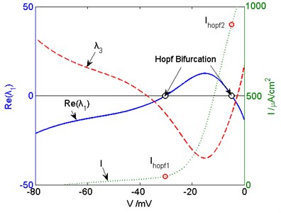
Fig. 2The eigenvalue and external input curves in the critical Hopf bifurcation point. The real part of λ1, λ3, and I are indicated by blue solid, red dashed, and green dotted lines, respectively

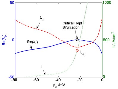
Fig. 1 shows the eigenvalue curves and external current of the three-dimensional Prescott model. It can be seen from the figure that the real eigenvalue ${\lambda }_3<0$ when the real part of the conjugate eigenvalues $\mathrm{R}\mathrm{e}\left({\lambda }_1\right)=0$. Therefore, the two intersections of $\mathrm{R}\mathrm{e}\left({\lambda }_1\right)$ curve and lateral axis are Hopf Bifurcation points of the model. The values of the first intersection are $V=\mathrm{}$–30.16 mV, $I=\mathrm{}$66.12 μA/cm².

The key parameter ${\beta }_w$ has a crucial impact on Hopf bifurcation of the model. Hopf bifurcation points change when ${\beta }_w$ has different values. When the $\mathrm{R}\mathrm{e}\left({\lambda }_1\right)$ curve is tangent to lateral axis, which is shown in Fig. 2, there is only one Hopf bifurcation point. If Hopf bifurcation no longer happens in the model when ${\beta }_w$ is smaller than a certain value, we call the certain value critical Hopf bifurcation point in this paper.

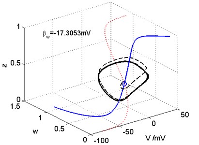
The values in the critical Hopf bifurcation point are ${\beta }_w=\mathrm{}$–17.3053 mV, $V_{Ho}=\mathrm{}$–22.84 mV. The $V$ nullcline, $w$ nullcline, phase trajectories of the three-dimensional Prescott model are shown in Fig. 3, we can see from the figure that the initial value starts from the Hopf bifurcation point, moves along a closed trajectory, and finally reaches on a stable closed track.

Fig. 3The phase space in the critical Hopf bifurcation point. The V nullcline, w nullcline, and phase trajectories are indicated by blue solid, red dotted, and black dashed lines, respectively

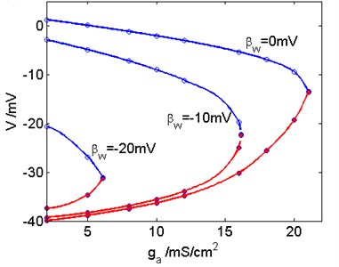
Adaptation plays a vital role in the information processing of neurons. Now we analyze the influence of the adaptive current and key parameter ${\beta }_w$ on Hopf bifurcation. When the conductance of adaptive current $g_a$ has different values, the changes of Hopf bifurcation points with ${\beta }_w$ are shown in Fig. 4(a). With $g_a$ increasing, the value of ${\beta }_w$ in the critical Hopf bifurcation point increases as well. On the other hand, when the values of ${\beta }_w$ are different, Hopf bifurcation points of the model varying with $g_a$ are depicted in Fig. 4(b). With ${\beta }_w$ growing, the value of $g_a$ in the critical Hopf bifurcation point also increases.

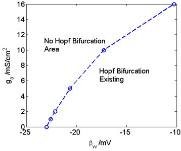
Therefore, ${\beta }_w$ and $g_a$ together affect the generation of the critical Hopf bifurcation. In the $g_a$-${\beta }_w$ plane, the critical Hopf bifurcation curve are drawn in Fig. 5. The left side of the dividing line does not exist Hopf bifurcation, that is, no matter how much the external current is, Hopf bifurcation will not occur. On the right side of the dividing line, Hopf bifurcation can occur in the three-dimensional Prescott model.

Fig. 4a) The Hopf bifurcation points vary with βw when ga is different; b) The Hopf bifurcation points vary with ga when βw is different

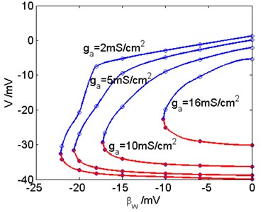
a)

b)

3. Judging the Hopf bifurcation type of three-dimensional Prescott model

Consider a three-dimensional nonlinear system:

where $\mathbf{x}$ is the state vector, $\mu \in R$ is bifurcation parameter. Let $\dot{\mathbf{x}}=\mathbf{f}(\mathbf{x},\mu )=0$, find the equilibrium point ${\mathbf{x}}_0\left({\mu }_0\right)=\left[x_{10}\right({\mu }_0),x_{20}({\mu }_0),x_{30}({\mu }_0){]}^T$. Extract the linear portion, and the equation can be rewritten as:

where $\mathbf{A}$ is the Jacobian matrix of the equilibrium point, $\mathbf{g}\left(\mathbf{x}\right)$ is nonlinear term:

Fig. 5The critical Hopf bifurcation curve in the ga-βw plane

Take linear transformation for the three-dimensional system: $\mathbf{x}=\mathbf{P}\mathbf{y}+{\mathbf{x}}_0\left({\mu }_0\right)$, where $\mathbf{P}=\left[\begin{array}{lll}\mathrm{R}\mathrm{e}\left({\lambda }_1\right)& \mathrm{I}\mathrm{m}\left({\lambda }_1\right)& {\lambda }_3\end{array}\right]$. The first two columns of $\mathbf{P}$ are the real and imaginary parts of the eigenvector corresponding to eigenvalue ${\lambda }_1=i{\omega }_0\left(\mu \right)$ of $\mathbf{A}$. The third column of $\mathbf{P}$ is the eigenvector corresponding to the real root ${\lambda }_3$. Therefore:

where $\mathbf{J}={\mathbf{P}}^{-1}\mathbf{A}\mathbf{P}$ is the Jordan matrix of the system, $\mathbf{F}={\mathbf{P}}^{-1}\mathbf{f}(\mathbf{P}\mathbf{y}+{\mathbf{x}}_0({\mu }_0\left)\right)-\mathbf{J}\mathbf{y}$ is nonlinear term:

The type of Hopf bifurcation can be determined according to the high dimensional Hopf bifurcation theory [22]:

It can be simplified to:

with:

As for three-dimensional system, $n=\mathrm{}$3, so:

with:

where ${\lambda }_3$ is the real eigenvalue of the equilibrium point, ${\omega }_0>0$ is the imaginary part of the purely imaginary characteristic roots. Therefore, the judgement formula of the Hopf bifurcation type of three-dimensional model is:

When ${\beta }_2>0$, subcritical Hopf bifurcation occurs, the new equilibrium branch is unstable when the bifurcation parameter is greater than the bifurcation value. When ${\beta }_2<0$, supercritical Hopf bifurcation occurs, a stable equilibrium point becomes an unstable equilibrium point and produces a stable limit cycle when the bifurcation parameter changes to the bifurcation value. The new equilibrium branch is stable when the bifurcation parameter is greater than the bifurcation value.

As for the three-dimensional Prescott model, ${\mathbf{x}}_0=(V_0,w_0,z_0)$, ${\mu }_0=I_0$, we can deduce the nonlinear term $\mathbf{f}(\mathbf{P}\mathbf{y}+{\mathbf{x}}_0({\mu }_0\left)\right)$ in $\mathbf{F}$:

The external current in Hopf bifurcation point is $I=\mathrm{}$42.94 μA/cm², Hopf bifurcation point is $(V_0,w_0,z_0)=(-\mathrm{39.2767,0.0029,0.0804})$. The matrix $\mathbf{P}$ in Hopf bifurcation point is:

Then we can calculate ${\mathbf{P}}^{-1}$, and $\mathbf{F}={\mathbf{P}}^{-1}\mathbf{f}(\mathbf{P}\mathbf{y}+{\mathbf{x}}_0({\mu }_0\left)\right)$ can be obtained. Use Eq. (20), ${\beta }_2=\mathrm{}$0.001765 > 0 can be calculated. Thus subcritical Hopf bifurcation occurs in the model. As the bifurcation parameter $I$ increases, an unstable limit cycle shrinks to an equilibrium and makes it lose stability. The subcritical Hopf bifurcation of the three-dimensional Prescott model before control is shown in Fig. 6. It can be seen from the figure that the stable equilibrium loses its stability when the external current $I=\mathrm{}$42.94 μA/cm².

Fig. 6The subcritical Hopf bifurcation occur in the Prescott model before control

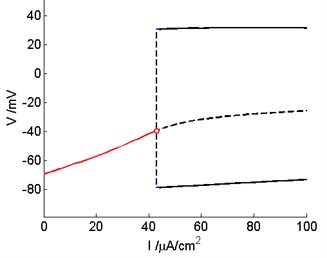
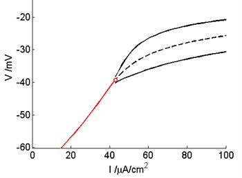
Fig. 7The supercritical Hopf bifurcation occur in the Prescott model after control with Washout filter

4. The control of Hopf bifurcation type using Washout filter

Subcritical Hopf bifurcation causes the new equilibrium branch of the system to lose stability. To avoid this happening, this paper design the controller based on Washout filter for subcritical Hopf bifurcation caused by the bifurcation parameter $I$. Since adding the controller does not change the equilibrium position of the system, so as not to change the operating state of the system, thus to avoid waste of energy, we choose Washout filter to control the Hopf bifurcation type of neuron model. The dynamic equations after joining the controller are as follows:

where $u$ is the nonlinear Washout controller, $v$ is the state variable of the controller, $k$ is the gain of the Washout controller, and $\xi$ is the inverse of the time constant, which is set to 0.5 in this paper.

From Eq. (14) we know, as for four-dimensional system, $n=4$, $\mathrm{R}\mathrm{e}\left(2G_{110}^2{w}_{11}^2\right)$ and $\mathrm{R}\mathrm{e}\left(G_{101}^2{w}_{20}^2\right)$ are needed to calculate Hopf bifurcation type judgement formula:

When the external current is $I=\mathrm{}$42.94 μA/cm², the Hopf bifurcation point is $(V_0,w_0,z_0,v_0)=(-\mathrm{39.2767,0.0029,0.0804},-78.5533)$. We can calculate and obtain the formula ${\beta }_2=-0.074957734k-0.00051748551$ from Eqs. (20), (25-26). When $k<\mathrm{}$–0.0069, ${\beta }_2<\mathrm{}$0. Therefore, the Hopf bifurcation of the model is supercritical Hopf bifurcation at $I=\mathrm{}$42.94 μA/cm² which is shown in Fig. 7.

5. Discussions

In this part, we will discuss how the presented method for controlling Hopf bifurcation of a single neuron could be used for a network of neurons. Here we consider a neural network of two coupled Prescott neurons, which can be described by the following equations:

where $g_{12}=g_{21}=g$ is the coupling strength, $f_{i1},f_{i2},f_{i3}\mathrm{}(i=1,\mathrm{}2)$ are depicted as follows:

The parameters of the two neurons are the same as presented in Section 2. Set ${\mathbf{x}}_{i0}=(V_{i0},w_{i0},z_{i0}{)}^T\mathrm{}(i=1,\mathrm{}2)$ to be the equilibrium points of the coupled neural network, the characteristic equation of the network is ${\left|\mathbf{B}-\lambda \mathbf{I}\right|}_{\mathbf{x}={\mathbf{x}}_{i0}}=0$, where $\mathbf{B}=\left[\begin{array}{ll}\mathbf{A}& \mathbf{G}\\ \mathbf{G}& \mathbf{A}\end{array}\right]$ is the coefficient matrix of the coupled system, and it is a real symmetric matrix:

According to the matrix block theory:

Expand Eq. (29) into characteristic polynomial:

where:

Although the characteristic matrix is six-dimensional for coupled three-dimensional Prescot neurons, it can be reduced to two three-dimensional determinant since the coupling terms are symmetric, and therefore simplifies the calculation.

According to the Routh-Hurwitz criterion [23], the system undergoes a Hopf bifurcation at $\mathbf{x}={\mathbf{x}}_0$$(\mu ={\mu }_0)$ if the following conditions are satisfied:

(1) Eigenvalue crossing condition:

(2) Transversality condition:

For $g=$ 0.5, the bifurcation points of Neron 1 are:

the bifurcation points of Neron 2 are:

The critical step for Hopf bifurcation control of the coupled neurons is to obtain the characteristic polynomial coefficients and then the Hopf bifurcation points. The coupled Prescott model is a six-order transcendental equation. The difficulty of bifurcation analysis for high-dimensional nonlinear equations is the dimensionality reduction. In this paper, we reduce the six-order characteristic polynomial to two three-order characteristic polynomials, and therefore determine the Hopf bifurcation points of the model. Next step, we can apply the technique proposed previously to judge Hopf bifurcation type of the network and control the Hopf bifurcation if it is subcritical Hopf bifurcation.

6. Conclusions

In this paper, we study the Hopf bifurcation characteristics of the three-dimensional Prescott neuron model, analyze the effect of adaptation conductance $g_a$ and ion channel key parameter ${\beta }_w$ on the critical Hopf bifurcation point, and obtain the region on $g_a$-${\beta }_w$ plane which Hopf bifurcation can occur. Using high-dimensional Hopf bifurcation theory, we derive the analytical formula for judging Hopf bifurcation type of three-dimensional nonlinear model, and judge the Hopf bifurcation type of the Prescott model via the formula. By applying a Washout filter to control the three-dimensional model, the Hopf bifurcation type of Prescott model is converted from subcritical Hopf bifurcation to supercritical Hopf bifurcation. The method for judging and controlling Hopf bifurcation type proposed here also applies to a network of two coupled Prescott neurons. The results in this paper provide theoretical foundations for biophysical dynamics of neurons and lighten a new way of treating neurological diseases such as Parkinson and epilepsy.