Vector matching-based disturbance rejection method for load simulator

1. Introduction

Load simulator is a kind of hardware-in-the-loop simulation equipment [1]. For the most part, they have three components: a loading system, a load-carrying object, a measuring-control system. The purpose of load simulation is to test the performance of a load-carrying object under the condition as real as possible. It helps designers to foresee and detect problems related to mechanics and control of the load-carrying object before it even is created, hence saving a lot of time and cost. There are many successful examples of the application of load simulators relate to aerospace [2, 3], robotics, mechatronics [4], automation [5] and other fields.

In the process of load simulation, a load-carrying object will be moving according to the test signal. For example, in the field of aerospace, the rudder actuator is often implemented as a load-carrying object. It must move, just like when the rocket is in the air. This motion is called as position disturbance. In this condition, the load simulator is not able to accurately control the loading force unless the control system takes the motion into account and makes an appropriate compensation. There are many kinds of position disturbance rejection methods. These methods can be divided into four categories, i.e., the position synchronization information feedforward method, the disturbance force/torque observation method, the composite control method and the disturbance model matching method.

Synchronization is the key to the first method. That is to say, if a loading system can be kept relatively static with a load-carrying object, disturbance torque could be eliminated completely. Under the guidance of this idea, researchers conducted a variety of attempts, including installing the loading motor on a position synchronous motor, as known as the hardware synchronous method [6]. To a certain extent, this method can eliminate the surplus torque caused by speed interference. It is suitable for low frequency and small amplitude disturbance case. But it also makes the system more complex, causes higher cost. In this respect, software synchronization method has obvious advantages. Among the software methods, structure invariance principle [7] is the most widely developed and has the most profound influence [8]. This principle is derived from invariance principle which was proposed by Soviet scholar Г. В. Щипанов in 1939 [9]. The author pointed out that, in a control system with external disturbances, the controller should be divided into two parts. One part is used to compensate the disturbance. The other is used to realize tracking. But all the rejection methods based on the structural invariance principle require a precise mathematical model of the system, which is hard to achieve.

The focus of the second method is concerned with disturbance torque itself. Fang Qiang proposed a disturbance observer design method for electric load simulator [10]. This observer can estimate generalized disturbance information which is a decoupling disturbance signal, through the disturbance torque and the loading command signal. This design makes great progress, considering uncertainties of the mathematical model. However, compared with the real disturbance, a time delay of the estimated disturbance is inevitable, making it difficult to completely eliminate the disturbance.

The characteristic of composite control strategy is that it is necessary to handle position synchronization information and feedback torque at the same time. The composite controller includes two parts. One part is an intelligent controller to eliminate the influence of position disturbance, and the other is a PID controller to ensure stability of the system during learning process of the intelligent controller. Neural networks [11], fuzzy logic [12] and iterative learning theory [13] are employed in the design of intelligent controllers. Although this method can deal with nonlinearity and uncertainty of the system, the convergence is still needed to be careful in.

The matching relation between position disturbance model and loading system model is what the last method looks for. A dynamic fuzzy neural network is applied to design the controller of load simulator [14, 15]. The idea of this method is to construct an inverse disturbance model, based on which a torque command to counteract the effect of position disturbance is generated. This is similar to the deconvolution method. However, it is hard to achieve due to the difficulty of the shock response acquisition, model uncertainty, nonlinearity and time variation. Robust methods and game theory have been used to solve the above problems [16, 17], and make deconvolution problem solved partly.

In summary, each of these methods has both advantages and disadvantages. Classical control theory is simple and powerful in form, but lack of adaptability. While modern control theory and intelligent control theory are enough to deal with complex problems, it is lack of stability and maneuverability. The key to success is to maximize the advantages of the method, according to the actual situation. For a load simulator, sine and square waves are the most widely used test commands of the load-carrying object. The common point is that these signals are cyclical. In this way, the test commands are able to be expanded into Fourier series, and each frequency component can be regarded as a signal vector.

Motivated by the above discussion, a new idea is presented in this paper, which is based on the matching relationship between load-carrying object position signal and torque signal of the loading system. Then, the matching problem of the disturbance model is simplified to a single or finite frequency sequence matching problem, called as vector matching problem. The critical part of the method is to find the relationship between the phase and amplitude of different signal vectors. This method is much easier to operate and needs no accurate mathematical model.

The rest of this paper is organized as follows. In Section 2, the structure of a load simulator and the principle of vector matching are introduced. The algorithm of vector matching-based disturbance rejection (VMBDR) method is presented in Section 3. In Section 4, some experiments are designed to verify the algorithm. Finally, results and further studies are discussed in the conclusion.

2. System description and vector matching principle

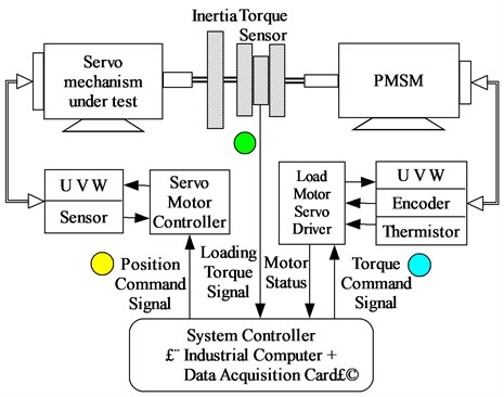
The electric load simulator (abbr. ELS) consists of three parts. 1) A servo mechanism under test, which is the actuator of a rudder in this experimental project, is used as the load-carrying object. It is connected to a torque sensor through a coupling. During the experiment, the servo mechanism rotates following the position commands. 2) A loading system, consisting of a PMSM and a motor driver, is connected to the torque sensor as well. 3) A measuring-control system mainly includes a torque sensor and an industrial computer with data acquisition cards, collecting the actual load torque in real time. The outputs of measuring-control system are angular displacement commands and loading system torque commands, respectively.

ELS is a typical double input and single output linear system. For a linear system, as showed in Fig. 1, use yellow on behalf of the position command signal and blue on behalf of the torque command signal, then the feedback loading torque signal should look like green. This is the superposition of linear systems, which is the basis of vector matching.

Fig. 1Construction diagram of an ELS

In order to explain the principle of vector matching, assume that the position command and the torque command are sinusoidal signals of the same frequency. These two commands generate two components of the resultant torque respectively. Fig. 2 shows the relationship between these three torque signals in polar coordinate system.

Fig. 2Schematic diagram of vector matching relation

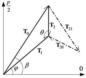
The symbols in Fig. 2 are defined as follows:

${\mathbf{T}}_0$ – resultant torque vector measured by the torque sensor,

${\mathbf{T}}_1$ – torque vector produced by the movement of the load-carrying object,

${\mathbf{T}}_2$ – torque vector produced by the loading system under the torque command ${\mathbf{T}}_{\mathrm{c}}$,

${\mathbf{T}}_{20}$ – one component of ${\mathbf{T}}_2$,

${\mathbf{T}}_{21}$ – another component of ${\mathbf{T}}_2$,

$\beta$ – phase angle of ${\mathbf{T}}_0$,

$\phi$ – phase angle of ${\mathbf{T}}_1$,

$\theta$ – angle between ${\mathbf{T}}_1$ and ${\mathbf{T}}_2$.

According to the invariance principle, ${\mathbf{T}}_{\mathrm{c}}$ should consist of two parts, i.e. ${\mathbf{T}}_{\mathrm{c}}={\mathbf{T}}_{\mathrm{c}0}+{\mathbf{T}}_{\mathrm{c}1}$. ${\mathbf{T}}_{\mathrm{c}0}$ is used to compensate for the position disturbance, and ${\mathbf{T}}_{\mathrm{c}1}$ is used to realize the loading. The purpose of vector matching is to make ${\mathbf{T}}_{20}\mathrm{}$equal to ${-\mathbf{T}}_1$.When the load target is 0 Nm, ${\mathbf{T}}_{21}$ should be equal to 0, and ${\mathbf{T}}_2$ should be equal to ${-\mathbf{T}}_1$.

Therefore, the vector relation described in Fig. 2 is the basic of the vector matching method, from which we can see that obtaining the angle $\theta$ is the key of vector matching. Fig. 3 demonstrates the working principle of VMBDR for ELS. Some symbols are defined in the figure and the others are defined as follows:

$L_{\mathrm{m}}$ – Motor stator cyclic inductance,

$R_{\mathrm{m}}$ – Motor stator resistance,$\mathrm{}$

$J_{\mathrm{m}}$ – Moment of inertia on the motor shaft,

$B_{\mathrm{m}}$ – Viscous friction coefficient on motor shaft,

$K_{\mathrm{e}}$ – Back EMF coefficient,$\mathrm{}$

$K_{\mathrm{t}}$ – Torque coefficient,$\mathrm{}$

$U$ – Armature voltage,

$E$ – Back- EMF,

$I^{\mathrm{*}}$ – Current command,

$i$ – Armature current,

$T_{\mathrm{L}}$ – Output load torque,

${\theta }_{\mathrm{o}\mathrm{u}\mathrm{t}}$ – Elastic deformation of the shaft.

Fig. 3VMBDR of the electric load simulator

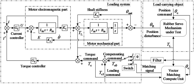
As shown in Fig. 3, the vector matching process is divided into three basic steps. The first two steps are the initialization of VMBDR. Its purpose is to gather the necessary information for step 3, i.e., the amplitude and phase of ${\mathbf{T}}_1$ and ${\mathbf{T}}_2$.

In the control system, there is a switch, which makes the control work in accordance with steps of 1, 2 and 3. In order to facilitate description, set the loading command $T_{\mathrm{c}1}$ to 0 Nm at first. Then, when the switch is at position 1, the compensating signal $T_{\mathrm{c}0}$ is zero, and the original position disturbance torque vector ${\mathbf{T}}_1$ could be obtained. As the switch is at position 2, the compensating signal $T_{\mathrm{c}0}$ is a filtered position command ${\theta }_{\mathrm{c}}$, and the resultant torque vector ${\mathbf{T}}_0$ could be gotten. Usually, the filter is a proportion link. So far, vector matching unit uses ${\mathbf{T}}_0$ and ${\mathbf{T}}_1$ to compute the loading torque vector ${\mathbf{T}}_2$ and $\theta$, then calculates a new compensating signal, which can eliminate ${\mathbf{T}}_1$ completely in step 3.

Changes in the environment will affect many physical parameters of ELS – motor stator resistance$R_{\mathrm{m}}$, for instance. This effect cannot be ignored when the test time is long enough, although this process is usually slow. Therefore, the control error of ${\mathbf{T}}_{20}-{\mathbf{T}}_1$ should be monitored in real time, and ${\mathbf{T}}_{20}$ should be fine-tuned by vector matching unit, when the error is accumulated to a certain extent.

Noise is another factor which has a great influence on the accuracy of vector matching, in addition to the parameter variability. The three inputs of the vector matching unit are torque command $T_{\mathrm{c}}$, position command ${\theta }_{\mathrm{c}}$ and output load torque $T_{\mathrm{L}}$ measured by the torque sensor, as shown in Fig. 3. $T_{\mathrm{c}}$ and ${\theta }_{\mathrm{c}}$ are generated by ELS controller computer itself. So only $T_{\mathrm{L}}$ could be contaminated by the additive noise. A Butterworth filter could be used to process the contaminated $T_{\mathrm{L}}$, when the noise is too large. However, the influence of the filter on the position disturbance torque vector ${\mathbf{T}}_1$ and the loading torque vector ${\mathbf{T}}_2$ are the same. Therefore, the matching relation between ${\mathbf{T}}_1$ and ${\mathbf{T}}_2$ does not change.

3. Vector-matching algorithm

ELS is a typical double input linear system. For a linear system, the output torque should obey the principle of superposition. So transfer function of the $T_{\mathrm{L}}$ is:

In the following, $W_{\mathrm{M}}\left(s\right)$ and $W_{\mathrm{R}}\left(s\right)$ are called non-disturbing load transfer function and position disturbance transfer function, respectively. Their frequency domain expressions are described as:

Assuming there is a sinusoidal position disturbance $\sin \left(\omega t\right)$. When the loading command $T_{\mathrm{c}1}$ is equal to 0 Nm, the output torque is only $T_1$, and $T_1=A_{\mathrm{R}}\left(\omega \right)\sin \left[\omega t+{\phi }_{\mathrm{R}}\left(\omega \right)\right]$. The total output $T_{\mathrm{L}}$ is expected to be 0 Nm. Thus, according to the principle of vector matching and the frequency characteristics of the model, a torque command could be constructed as follows:

So the core of VMBDR is to identify the amplitude and phase of each vector signal. There are two kinds of VMBDR algorithms, corresponding to the sine position disturbance and the other periodic position disturbance respectively.

3.2. Complex vector matching algorithm

While the position disturbance is a non-sinusoidal periodic signal, complex vector matching algorithm (abbr. CVM) could be used. Although the Fourier series of the periodic signal includes infinite harmonic components, in practice, the load simulator is equivalent to a low pass filter. Thus the disturbance signal only retains a finite number of harmonic components. Batch processing of a finite number of vectors is realizable. This algorithm is an off-line identification algorithm based on FFT and IFFT.

The basic idea of CVM is consistent with SVM. The difference is that CVM works in the complex domain. The process of CVM is illustrated in Fig. 4.

Fig. 4Principle diagram of the complex vector matching method

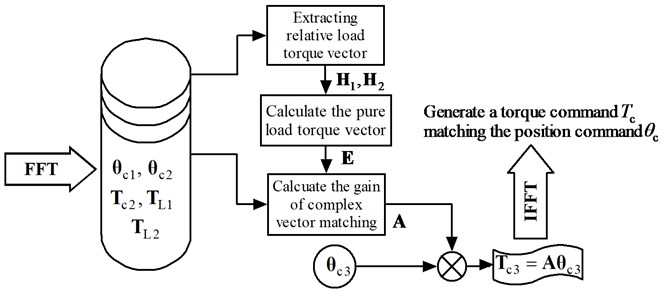
Fig. 4 introduces a number of vector symbols as follows (n is the length of FFT). Each of them represents a Fourier transform of a signal. Each of the elements in the vectors is written in complex index form.

${\mathbf{\theta }}_{\mathrm{c}1}={\left({\theta }_{\mathrm{c}11},{\theta }_{\mathrm{c}12},\cdots ,{\theta }_{\mathrm{c}1n}\right)}^{\mathrm{T}}$ – Position command complex vector in step 1,

${\mathbf{\theta }}_{\mathrm{c}2}={\left({\theta }_{\mathrm{c}21},{\theta }_{\mathrm{c}22},\cdots ,{\theta }_{\mathrm{c}2n}\right)}^{\mathrm{T}}$ – Position command complex vector in step 2,

${\mathbf{\theta }}_{\mathrm{c}3}={\left({\theta }_{\mathrm{c}31},{\theta }_{\mathrm{c}32},\cdots ,{\theta }_{\mathrm{c}3n}\right)}^{\mathrm{T}}$ – Position command complex vector in step 3,

${\mathbf{T}}_{\mathrm{c}2}={\left(T_{\mathrm{c}21},T_{\mathrm{c}22},\cdots ,T_{\mathrm{c}2n}\right)}^{\mathrm{T}}$ – Compensating command complex vector in step 2,

${\mathbf{T}}_{\mathrm{c}3}={\left(T_{\mathrm{c}31},T_{\mathrm{c}32},\cdots ,T_{\mathrm{c}3n}\right)}^{\mathrm{T}}$ – Compensating command complex vector in step 3,

${\mathbf{T}}_{\mathrm{L}1}={\left(T_{\mathrm{L}11},T_{\mathrm{L}12},\cdots ,T_{\mathrm{L}1n}\right)}^{\mathrm{T}}$ – Output load torque complex vector in step 1,

${\mathbf{T}}_{\mathrm{L}2}={\left(T_{\mathrm{L}21},T_{\mathrm{L}22},\cdots ,T_{\mathrm{L}2n}\right)}^{\mathrm{T}}$ – Output load torque complex vector in step 2,

${\mathbf{H}}_1={\left(H_{11},H_{12},\cdots ,{\mathrm{H}}_{1\mathrm{n}}\right)}^{\mathrm{T}}$ – Relative load torque complex vector in step 1,

${\mathbf{H}}_2={\left(H_{21},H_{22},\cdots ,{\mathrm{H}}_{2\mathrm{n}}\right)}^{\mathrm{T}}$ – Relative load torque complex vector in step 2,

$\mathbf{E}={\left(E_1,E_2,\cdots ,{\mathrm{E}}_{\mathrm{n}}\right)}^{\mathrm{T}}$ – Pure load torque complex vector in step 2,

$\mathbf{A}={\left(A_1,A_2,\cdots ,A_n\right)}^{\mathrm{T}}$ – Gain of complex vector matching used in step 3.

In step 1 the compensation command is zero, so ${\mathbf{T}}_{\mathrm{L}1}$ contains the position disturbance torque only. However, in step 2, the compensation command is ${\mathbf{T}}_{\mathrm{c}2}$, then ${\mathbf{T}}_{\mathrm{L}2}$ turns out to be:

13

${\mathbf{T}}_{\mathrm{L}2}=W_{\mathrm{R}}\left(jk{\omega }_0\right){\mathbf{\theta }}_{\mathrm{c}2}+W_{\mathrm{M}}\left(jk{\omega }_0\right){\mathbf{T}}_{\mathrm{c}2}$
$\mathbf{}\mathbf{}\mathbf{}\mathbf{}\mathbf{}\mathbf{}\mathbf{}=A_{\mathrm{R}}\left(k{\omega }_0\right)A_{\mathrm{\theta }2}\left(k{\omega }_0\right)e^{j\left[{\phi }_{\mathrm{R}}\left(k{\omega }_0\right)+{\phi }_{\mathrm{\theta }2}\left(k{\omega }_0\right)\right]}+A_{\mathrm{M}}\left(k{\omega }_0\right)A_{\mathrm{T}2}\left(k{\omega }_0\right)e^{j\left[{\phi }_{\mathrm{M}}\left(k{\omega }_0\right)+{\phi }_{\mathrm{T}2}\left(k{\omega }_0\right)\right]},$
$k=\mathrm{1,2},\cdots ,n$

The object of complex vector matching is to construct a torque command vector, so that the error torque is close to zero in step 3. Thus, Eq. (14) should be satisfied.

14

$0=W_{\mathrm{R}}\left(jk{\omega }_0\right){\mathbf{\theta }}_{\mathrm{c}3}+W_{\mathrm{M}}\left(jk{\omega }_0\right){\mathbf{T}}_{\mathrm{c}3}.$

The key to achieve the complex vector matching is to obtain $W_{\mathrm{R}}\left(jk{\omega }_0\right)$ and $W_{\mathrm{M}}\left(jk{\omega }_0\right)$, which is essentially a model matching problem. Reference Eq. (13) and Eq. (14), the vector matching relationship can be described as follows:

15

${\mathbf{T}}_{\mathrm{c}3}=-\frac{W_{\mathrm{R}}\left(jk{\omega }_0\right)}{W_{\mathrm{M}}\left(jk{\omega }_0\right)}{\mathbf{\theta }}_{\mathrm{c}3}=-\frac{\frac{{\mathbf{T}}_{\mathrm{L}1}}{{\mathbf{\theta }}_{\mathrm{c}1}}{\mathbf{T}}_{\mathrm{c}2}}{\left(\frac{{\mathbf{T}}_{\mathrm{L}2}}{{\mathbf{\theta }}_{\mathrm{c}2}}-\frac{{\mathbf{T}}_{\mathrm{L}1}}{{\mathbf{\theta }}_{\mathrm{c}1}}\right)}{\mathbf{\theta }}_{\mathrm{c}3}=-\frac{{\mathbf{H}}_1{\mathbf{T}}_{\mathrm{c}2}}{\left({\mathbf{H}}_2-{\mathbf{H}}_1\right){\mathbf{\theta }}_{\mathrm{c}2}}{\mathbf{\theta }}_{\mathrm{c}3}=-\frac{{\mathbf{H}}_1{\mathbf{T}}_{\mathrm{c}2}}{\mathbf{E}{\mathbf{\theta }}_{\mathrm{c}2}}{\mathbf{\theta }}_{\mathrm{c}3}=\mathbf{A}{\mathbf{\theta }}_{\mathrm{c}3}.$

Eq. (15) shows the calculation process of the matching compensation torque command ${\mathbf{T}}_{\mathrm{c}3}$. Normally, rudder position command ${\mathbf{\theta }}_{\mathrm{c}3}$ is set in advance, according to experimental requirements. Once the complex gain vector $\mathbf{A}$ is determined, the compensation torque command ${\mathbf{T}}_{\mathrm{c}3}$ can be matched successfully.

The Fourier series of a periodic signal is a discrete sequence, and the non-zero components only exist on the harmonic frequencies of the periodic signal. Hence the actual calculation procedure of CVM is as follows:

16

$H_{ik}=\left\{\begin{array}{ll}\frac{T_{\mathrm{L}ik}}{{\theta }_{\mathrm{c}ik}},& {\theta }_{\mathrm{c}ik}\ne 0,\\ 0,& {\theta }_{\mathrm{c}ik}=0,\end{array}\right.$

17

$E_k=H_{2k}-H_{1k},$

18

$A_k=\left\{\begin{array}{ll}-\frac{H_{1k}{\theta }_{\mathrm{c}2k}}{E_k{T}_{\mathrm{c}2k}},& E_k\ne 0\text{and}{T}_{\mathrm{c}2k}\ne 0,\\ 0,& E_k=0\text{or}{T}_{\mathrm{c}2k}=0,\end{array}\right.$
$i=\mathrm{1,2},k=\mathrm{1,2},\cdots ,n.$

As shown in Eq. (16) to Eq. (18), only the components of harmonic frequencies are involved in the CVM operation. On the other hand, the noise components are distributed on the spectrum weakly and evenly, when the ELS has some measures to resist interference. Therefore, the effect of noise on the CVM operation is limited.

4. Experiment

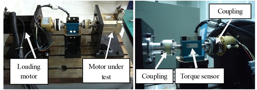
Experiments are carried out on a servo motor limit capacity test bench, shown in Fig. 5. Similar to the structure described in Fig. 1, the test bench mainly includes a loading motor, a motor under test which is the load-carrying object, and a torque sensor. Meanwhile, the torque sensor is grounded and isolated to reduce the influence of electromagnetic interference on torque measurement.

Fig. 5Photos of servo motor limit capacity test bench

The experiments including three sub-experiments could be divided into two categories. One is constant torque loading test, which means that the loading motor should load a constant torque on the motor under test. The loading torque is independent from the motion of the motor under test. The other is called as spring torque loading test. In this experiment, the loading motor is supposed to provide a torque proportional to the rotation angle of the motor under test. So the loading motor operates like a spring for the tested motor. Table 1 shows the arrangement of these experiments.

4.1. Sinusoid position – constant torque loading

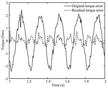
In this experiment, position command of the tested motor is a series of sinusoidal signals with the frequencies of 5 Hz, 10 Hz, 15 Hz. Control object of load torque is 0 Nm. Fig. 6, Fig. 7, and Fig. 8 demonstrate that, by using SVM, the residual torque error is obviously smaller than the original torque error. Detail data are provided in Table 2.

Fig. 65 Hz sinusoid position disturbance constant torque load curve

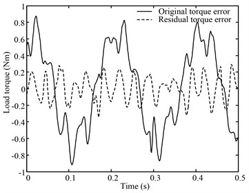
Fig. 710 Hz sinusoid position disturbance constant torque load curve

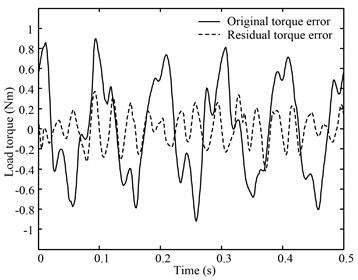
Fig. 815 Hz sinusoid position disturbance constant torque load curve

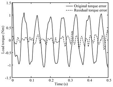
Table 2The detail data of the 1st experiment

Frequency (Hz)	Original torque standard deviation (Nm)	Residual torque standard deviation (Nm)	Elimination %
5	0.48954	0.14467	70.45
10	0.48782	0.17098	64.96
15	0.72031	0.12330	82.88

4.2. Triangle position – constant torque loading

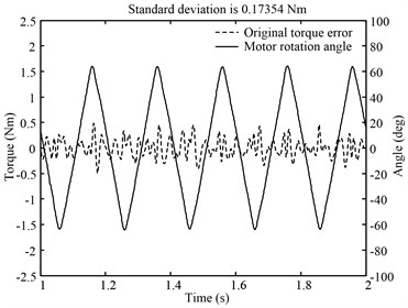
A 5 Hz triangle signal $x\left(t\right)$, whose magnitude is represented by $A_{\mathrm{t}\mathrm{r}\mathrm{i}}$, is adopted as the position command for the tested motor in this experiment. The Fourier series of $x\left(t\right)$ is shown in Eq. (19). CVM is utilized to improve the loading precision. By comparing Fig. 9 and Fig. 10, we can find that CVM greatly reduces the torque control error.

19

$x\left(t\right)=\frac{8A_{\mathrm{t}\mathrm{r}\mathrm{i}}}{{\pi }^2}\left[\cos \left({\omega }_{0}t\right)+\frac{1}{3^2}\cos \left(3{\omega }_{0}t\right)+\frac{1}{5^2}\cos \left(5{\omega }_{0}t\right)+\cdots \right]=\frac{8A_{\mathrm{t}\mathrm{r}\mathrm{i}}}{{\pi }^2}\sum _{n=1}^{\infty }\left[\frac{1}{n^2}\cos \left(n{\omega }_{0}t\right)\right]$
$n=\mathrm{1,3},\mathrm{5,7},\cdots .$

Fig. 9Torque error caused by position disturbance of triangular wave

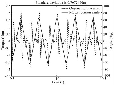
Fig. 10CVM effect of triangle wave position disturbance

Fourier transform of the test data illustrates the effect of CVM more intuitively. Fig. 11 shows amplitude spectrum of main signals, including the position command ${\mathbf{\theta }}_{\mathrm{c}3}$, the compensation torque command ${\mathbf{T}}_{\mathrm{c}3}$, the original torque error and the residual torque error. The effect of CVM is expressed numerically in Table 3.

Fig. 11Spectrum of triangular disturbance rejection experimental data

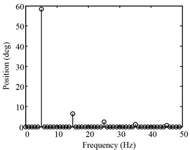
a) Position command

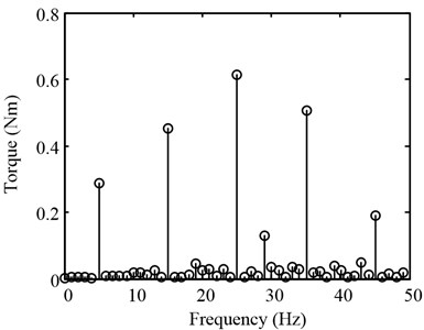
b) Original torque error

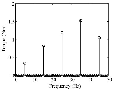
c) Matching torque command

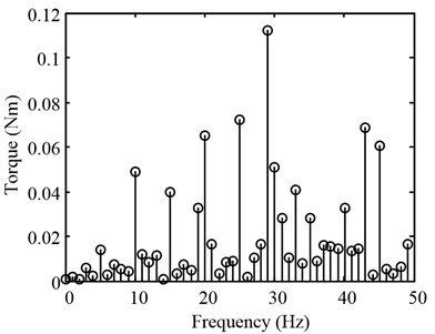
d) Residual torque error

Table 3Rejection effect of disturbance torque at each frequency component

Frequency (Hz)	Original torque standard deviation (Nm)	Residual torque standard deviation (Nm)	Elimination %
5	0.287	0.014	95.135
15	0.452	0.040	91.230
25	0.613	0.072	88.217
30	0.507	0.028	94.407
45	0.190	0.060	68.163

4.3. Sinusoid position – spring torque loading

In this experiment, position command of the tested motor is a 5 Hz sinusoidal signals. And loading motor must provide a load torque, with a load gradient of 0.05 Nm/deg. Fig. 12 shows that when only the feedback controller is working, load torque is obviously lagging behind the rotation of the tested motor. As demonstrated in Fig. 13, load torque and motor rotation are basically synchronous after applying the vector matching algorithm. The original torque error displays in Fig. 14 including two parts. One results from the lag of loading system. The other is caused by the position disturbance coming from the tested motor. Fig. 14 shows that VMBDR is highly effective at suppressing the two kinds of loading errors. The standard deviation of the load torque before and after compensation is: 1.4536 Nm and 0.25432 Nm.

Fig. 125 Hz spring torque loading before vector matching

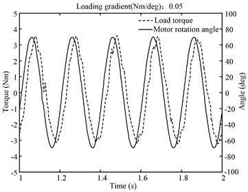
Fig. 135 Hz spring torque loading after vector matching

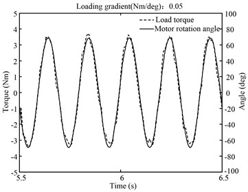
Fig. 14Error contrast before and after vector matching

5. Conclusion

Load simulator is a passive torque servo system and it is necessary to suppress the position disturbance. In this study, vector matching-based disturbance rejection (VMBDR) method is proposed. The effectiveness of the proposed algorithm is verified on an electric load simulator.

Single vector matching (SVM) method can eliminate sinusoidal position disturbance, and its elimination ratio is related to the precision of identification. Complex vector matching (CVM) method based on FFT can eliminate cyclical position disturbance. The experimental results show that elimination ratio of CVM is higher than SVM. In addition, the vector matching method can compensate the control error caused by the response lag of the loading system as well. This means that VMBDR is not only applicable to constant torque loading, but also to spring torque loading.

Finally, VMBDR works effectively on the electric load simulator which has high linearity. This suggests that, for other linear multi-input systems, vector matching method will be still effective in great probability.