Abstract
As the inclination of a bedding surface is consistent with the inclination of a slope, the stability of a bedding rock slope is relatively poor, especially under dynamic loads such as earthquake and blasting. In the dynamic stability analysis of slope, the evaluation methods and influence factors of slope stability are two important concerns. Therefore, two typical bedding rock slopes are respectively established by FLAC3D to study the above concerns. The pseudo-static method, dynamic time-history method and dynamic strength reduction method is used to evaluate the dynamic stability of the model slope, and the applicability of the three methods is compared. The influence of five parameters including dynamic load frequency, slope angle, slope height, strata inclination and strata thickness on the dynamic stability is considered in the model slope with a set of bedding planes. The results show that the dynamic strength reduction method has good suitability for the stability evaluation of a bedding rock slope due to its good solution in the instability judgment and evaluation index. The dynamic stability of a slope becomes worse when the load frequency is close to the natural frequency of the slope. Due to the “elevation effect” and “bedding surface effect” in the dynamic slope response, the slope stability decreases with the increase of slope height and the reduction of strata thickness. The slope stability decreases with the increase of strata inclination and slope angle, and the strata inclination is the most sensitive parameter influencing the slope stability. When the slope angle and height increase to a certain value, the downward trend of slope stability gradually become gentle. For the model slope in this paper, when the slope angle reaches 55° and the slope height reaches 200 m, the reduction of slope stability will be no longer obvious with the increase of a slope angle and slope height.
1. Introduction
Rock slope instability induced by earthquake and blasting is a common engineering geological hazard. The failure of rock slope under a dynamic load is characterized by sudden occurrence, strong damage and high speed movement and impact, which have caused great harm to human's living environment and engineering safety [1]. The dynamic stability of rock slope is mainly controlled by the internal structure surface, which is similar to that under static condition [2]. The bedding surface of rock slope is generally exposed in the slope surface and becomes a potential sliding surface. Under the action of earthquake and other dynamic loads, the layered rock mass may be destroyed along a certain bedding surface, leading to the instability of slope. Therefore, it is important to study the dynamic stability of bedding rock slope. Due to sudden destruction of the rock slope during an earthquake, it is difficult to observe the failure process in the actual condition. What’s more, the rock mass of slope after suffered earthquake action is extremely broken and usually shows the characteristics of high speed movement and remote accumulation, so that a large number of evidence to reflect the destruction process is covered. Therefore, a research on the failure mode and failure process of rock slope under dynamic load is usually carried out by shaking table test and numerical simulation. Fan G. et al. [3] and Xu Q. et al. [4] carried out a large-scale shaking table test to study the dynamic response of rock slope under seismic load. Fan G. et al. [5] discussed the dynamic response differences between bedding and count-tilt rock slopes with silted intercalation through a shaking table test. The numerical calculation method can well analyze the influence of seismic wave characteristics (such as frequency, duration, etc.) on the slope stability and accurately obtain the dynamic response slope characteristics, therefore it has gradually become one of the main methods to analyze the dynamic slope stability. The numerical analysis methods such as DDA, FLAC, PFC, and 3DEC have been widely used in the dynamic stability analysis of rock slope [6-9].
There are two main methods to evaluate the dynamic stability of rock slope, i.e. seismic permanent displacement method and dynamic stability coefficient method. In some literatures [10-12], the stability of a rock slope under the action of earthquake is evaluated by the permanent displacement method. However, this method is difficult to give a unified failure criterion, which is inconvenient to be used in practical engineering. The dynamic stability coefficient method can clearly give the slope stability index, so it is widely used in practical engineering. The dynamic stability coefficient method can be divided into the pseudo static method [13], dynamic time-history analysis method [14], and dynamic strength reduction method [15]. The pseudo static method transforms the seismic load into static action on the slope sliding body, and then carries out a limit equilibrium analysis. The dynamic time-history analysis method obtains the stability coefficient curve during an earthquake by calculating the slope stability at any moment of the earthquake action. The dynamic strength reduction method carries out a dynamic numerical calculation through the reduction of strength parameters. According to the corresponding critical state criterion, the reduction factor is used as the slope stability factor.
At present, the research on dynamic failure of bedding rock slope mainly focuses on two aspects: the dynamic response and stability evaluation of the slope. However, most of the dynamic stability evaluation methods for rock slope directly draw on the experience of the soil slope, which needs to be further studied on the suitability for the bedding rock slope. In addition, for this special structure type of rock slope, it is of a great significance to study the influence of slope geometry characteristics and dynamic load characteristics on slope stability. Based on this, this paper selects the bedding rock slope as the research object, uses FLAC3D to establish the numerical analysis model, and compares the suitability of three kinds of dynamic stability evaluation method in the bedding rock slope; secondly, the dynamic strength reduction method is used to analyze the influence factors of the dynamic stability of the bedding rock slope, and some meaningful conclusions are obtained.
2. Failure mode of bedding rock slope under dynamic load
2.1. Two typical failure modes
Strata inclination of bedding rock slope is usually consistent with slope inclination. According to the relationship between slope angle () and strata inclination (), it can be divided into two categories, i.e.: a) . The bedding surface is exposed in slope surface, and the stability of this type of slope is relatively poor, especially when the strata inclination is steep; For b) , it is difficult to form a continuous sliding surface, this kind of slope is usually stable under static condition.
According to the investigation of geological hazards in the Wenchuan Earthquake in China, the bedding rock slope under strong earthquake exhibited very poor stability, and a lot of large-scale landslides, such as the Tangjiashan landslide, Daguangbo landslide, Ganmofang landslide, Xinzhong landslide, and Xiaojiaqiao landslide etc., are all bedding rock slopes. Based on the analysis of instability cases of bedding rock slope caused by the Wenchuan earthquake, there are two typical failure modes of bedding rock slope under earthquake: a) sliding-fracturing failure, and b) sliding-bending failure. Normally, the first failure mode mainly appears in the slope with gently strata inclination, and the bedding surface is exposed in the slope surface (). The second failure mode mainly appears in the slope with a steep bedding surface, and the strata inclinationis usually greater than the slope angle (). Taking Daguangbao landslide and Ganmofang landslide, for example, two typical failure modes are illustrated as follows.
2.1.1. Sliding-fracturing failure
According to the deformation and failure of the Daguangbao landslide, its formation mechanism can be divided into several stages as shown in Fig. 1(a). At this stage, tension cracks begin to appear on the trailing edge of the landslide, and the crack depth increases continuously; Moreover, the bottom sliding surface tends to exhibit creeping deformation (Fig. 1(b)). At this stage, the trailing of landslide is completely pulled apart, and the fracture surface and sliding surface are linked into one. The landslide mass tends to perform integral sliding (Fig. 1(c)) When the mass slides to the valley bottom with a high speed, it will be braked by the mountain from the other side of the valley (Fig. 1(d)). When the slip-mass gradually tends to be still, the covering layer on its upper part will slip a second time under inertia force.
Fig. 1Failure mechanisms of Daguangbao landslide [16]
![Failure mechanisms of Daguangbao landslide [16]](https://static-01.extrica.com/articles/17210/17210-img1.jpg)
a) Initial vibration cracking
![Failure mechanisms of Daguangbao landslide [16]](https://static-01.extrica.com/articles/17210/17210-img2.jpg)
b) Trailing edge pulled off and sliding body start-up
![Failure mechanisms of Daguangbao landslide [16]](https://static-01.extrica.com/articles/17210/17210-img3.jpg)
c) High speed and braking by overlap
![Failure mechanisms of Daguangbao landslide [16]](https://static-01.extrica.com/articles/17210/17210-img4.jpg)
d) Secondary sliding stage
2.1.2. Sliding-bending failure
According to the failure characteristics of the Ganmofang landslide, its formation mechanism can be divided into the following stages. a) Stage of slippage along bedding as shown in Fig. 2(a). Due to the inertia force induced by the earthquake, the sliding body begins to move along the steep bedding plane. However, for the bedding surface is not exposed in slope surface, the sliding movement will be blocked by the middle and lower part of the slope. A “locking section” will be formed at the slope toe; b) Yield and bending stage of rock in “locking section” as shown in Fig. 2(b). With the continuous action of seismic load, further sliding movement of the upper rock mass leads to the stress concentration of the “locking section” in the middle and lower part of the slope. Therefore, the rock stratum is pressed and bent, resulting in the deformation of the bending and folding; c) Failure stage with perforation of sliding surface as shown in Fig. 2(c). The bend and uplift deformation of the middle and lower part of the slope accumulates with the vibration process, which eventually leads to the rock strata’s completely buckling. A shear zone with a low angle is formed, and a through sliding surface composed by a shear zone, and a sliding plane will be formed, which finally leads to the formation of the landslide.
Fig. 2Failure mechanisms of Ganmofang landslide [17]
![Failure mechanisms of Ganmofang landslide [17]](https://static-01.extrica.com/articles/17210/17210-img5.jpg)
a) Sliping along bedding surface and blocked by slope toe
![Failure mechanisms of Ganmofang landslide [17]](https://static-01.extrica.com/articles/17210/17210-img6.jpg)
b) Vibration intensified and “locking section” bending uplift
![Failure mechanisms of Ganmofang landslide [17]](https://static-01.extrica.com/articles/17210/17210-img7.jpg)
c) Uplift intensified and cut off causing formation of landslide
2.2. Differences between dynamic and static conditions in failure mode
Due to its special slope structure, the bedding rock slope can also undergo the instability just due to dead weight, water pressure, construction load and other factors under the static condition, especially when the bedding surface is exposed in the slope surface. However, considering that the seismic load has the characteristics of short duration and large force, the failure mode of the bedding slope under dynamic condition is different from that under the static condition. The main differences are as follows:
2.2.1. More instability cases of slope with steep bedding surface
Under the static condition, when the strata inclination () is larger than a slope angle (), the slope is usually stable due to the resistance provided by the rock mass at the slope toe. However, the rock mass at the slope toe may be crushed by the joint action of earthquake and gravity load, which ultimately lead to the overall slip of the upper rock mass. According to the landslide survey on the Wenchuan earthquake, a lot of instability cases of a slope with steep bedding surface () are found, as shown in Table 1. As can be seen from Table 1, the landslide quantity of slope with steep bedding surface accounts for almost half of the total number of bedding landslides. But the slope instability with a gentle and medial inclined bedding surface () is more common than that with steep bedding surface () under the static condition.
2.2.2. High and steep residual posterior wall
After the landslide of bedding rock induced be earthquake, there is usually a high and steep cliff left at the trailing edge of landslide as shown in Fig. 3, which is the main component of the sliding surface.
Different from the tension cracks formed by long-term geological action, the trailing cliff induced by seismic force has the larger scale and the characteristics of instantaneous rupture. This kind of tension crack usually extends through the weathered and fresh rock mass, exhibiting typical tensile failure characteristics.
Table 1Number of bedding rock slopes instability in study region [18]
Suishui river | Chaping river | Mianyuan river | Shiting river | |
Slopes with gentle inclined bedding surface | 10 | 0 | 0 | 16 |
Slopes with medial inclined bedding surface | 51 | 25 | 23 | 21 |
Slopes with steep inclined bedding surface | 19 | 18 | 67 | 27 |
Fig. 3Residual cliff at trailing edge of Daguangbao landslide [16]
![Residual cliff at trailing edge of Daguangbao landslide [16]](https://static-01.extrica.com/articles/17210/17210-img8.jpg)
2.2.3. Gentle shear section at leading edge
In addition to the steep trailing cliff mentioned above, some of large landslides at a high position also have a relatively gentle shear section at the leading edge. The sliding surface morphology under dynamic and static conditions is shown in Fig. 4. As it can be seen in Fig. 4, the sliding surface morphology of landslides induced by earthquake has a longer tension section and shorter shear section than that under the static condition.
Fig. 4Comparison of sliding surface morphology under dynamic and static conditions
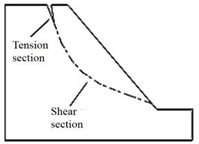
a) Static condition
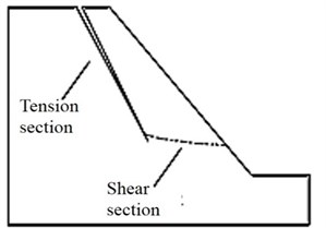
b) Dynamic condition
3. Evaluation methods of slope dynamic stability
A typical numerical simulation model of bedding rock slope is established by FLAC3D in this section. Three kinds of dynamic stability coefficient methods including the pseudo static method, dynamic time history analysis method and dynamic strength reduction method are adopted to evaluate the stability of the model slope under earthquake load.
3.1. Numerical analysis model
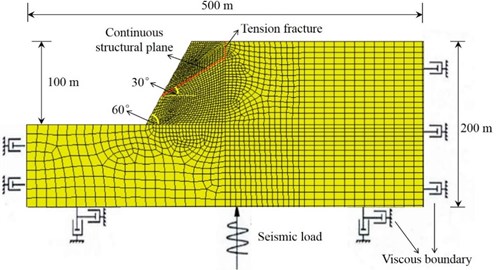
Numerical analysis model of the slope is shown in Fig. 5. The model is 500 m long and 200 m high. The slope is 100m high with a structural plane of 30° and a slope angle of 60°. Rock materials in the model are ideal elastic-plastic materials subject to the Mohr-Coulomb yield criterion, and the structural plane is simulated with contact elements subject to the Coulomb slide model. Limestone is used as the model material in the numerical calculation. Physic-mechanical parameters of rock material and structural plane are shown in Table 2 and Table 3. The viscous boundary is used as the dynamic boundary condition, and the local damping coefficient is 0.15.
Fig. 5Numerical analysis model
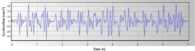
The acceleration-time curve of the Wenchuan Earthquake recorded by the Chengdu Station (CD2-BHE) (excluding the foreshock) was selected in this paper, and the wave section of 26 s-33 s was used as the waveform of a seismic wave. Also, reduction in the peak acceleration was conducted due to the poor stability of a numerical slope model to generate the acceleration-time curve. The processed seismic wave applied on the slope model is shown in Fig. 6. The peak acceleration is 0.34 m/s2, and the duration time is 7 s.
Table 2Physic-mechanical parameters of model rock
Density / kg·m-3 | Tensile strength / MPa | Cohesion / MPa | Friction angle / (°) | Elastic modulus / GPa | Poisson’s ratio | Damping ratio | |
Limestone | 2600 | 0.6 | 1 | 40 | 25 | 0.22 | 0.048 |
Table 3Mechanical parameters of structural plane
Tensile strength / MPa | Cohesion / MPa | Friction angle / (°) | Normal stiffness / GPa·m-1 | Tangential stiffness / GPa·m-1 | |
Continuous structural plane | 0.08 | 0.030 | 32 | 10.2 | 6.4 |
Tension fracture | 0.003 | 0.006 | 20 | 8.2 | 5.1 |
Fig. 6Time-history curve of acceleration (after filtering and baseline correction)
3.2. Pseudo-static method
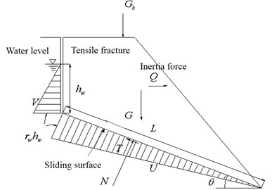
The pseudo-static method to evaluate the dynamic stability of slope mainly follows the idea of the limit equilibrium of rigid body. It simplifies the dynamic inertia force generated by the earthquake into the horizontal and vertical static force which is then applied to the barycenter of the sliding body. Then, based on the limit equilibrium theory, the stability coefficient of the slope is calculated. For the bedding rock slope, the calculation schematic diagram of pseudo-static methods shown in Fig. 7 when only considering the horizontal seismic force.
Fig. 7Calculation schematic diagram of pseudo-static method
The calculation formulas of the dynamic stability coefficient of the slope can be obtained as follows from Fig.7:
In the above equations, is the sliding force caused by unit width gravity of sliding body and other external force (kN/m); is the anti-slide force caused by the friction force and the cohesive force on the sliding surface and other external force (kN/m); is the effective cohesion of the sliding surface (kPa); is the effective internal friction angle of the sliding surface (°); is the length of the sliding surface (m); is the angle of the sliding surface (°); is the unit width weight of sliding body (kN/m); is the unit width vertical additional load of sliding body (kN/m); is the total water pressure on unit width of the sliding surface (kN/m); is the total water pressure on unit width of the steep fracture surface at the trailing edge; is the earthquake load on unit width of the sliding body (kN/m), and its direction is outside the slope, , where is the horizontal seismic coefficient.
As it can be seen from the calculation process, the dynamic seismic load is equivalent to the static load in the calculation of the stability coefficient. In essence, it still belongs to the static stability analysis method. Choosing a reasonable value to represent the seismic inertia force applied to the sliding body is the core of this method. In the practical application, the horizontal seismic coefficient “” usually takes 1/3 g times of the maximum acceleration during an earthquake, and the vertical seismic coefficient is the 2/3 times of horizontal seismic coefficient [19]. According to the geometric size of the slope, material parameters and peak acceleration of the dynamic load, the dynamic stability coefficient “” of the model slope is 1.24 which can be calculated by the Eqs. (1)-(3) (without considering the influence of ground water).
3.3. Dynamic time-history method
Dynamic time-history method is generally based on a dynamic numerical algorithm to obtain the dynamic stress field of the slope. Then according to the limit equilibrium theory, the time history curve of stability coefficient in the whole seismic duration is obtained by calculating the stability coefficient in each step. For the plane sliding failure mode, the instantaneous stability coefficient of the slope can be obtained by calculating the nodal force of the rock mass at any moment.
The nodal force is the joint force of the gravity and seismic inertia force of the rock mass at the moment of , and by projecting it along the potential sliding direction, the sliding force can be obtained as follows:
where, is the unit vector of potential sliding direction.
The normal counter-force on the sliding surface can be obtained by projecting into the normal direction of the sliding surface. According to the Coulomb friction law, the anti-sliding force is:
where, is the unit normal vector of the sliding surface; is the contact area between the sliding body and lower rock mass; and are respectively the internal friction angle and cohesion of sliding surface at the moment of .
Thus, the stability coefficient of the slope at any moment under earthquake action can be calculated as follows:
The calculation process of Eq. (8) can be realized by “fish” language programming in FLAC3D. The stability coefficient of the model slope calculated by Eq. (8) under the action of earthquake load is as shown in Fig. 8.
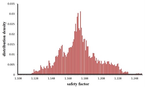
The time-history curve of the stability coefficient reflects the variation of the slope stability during an earthquake, but it cannot directly give an evaluation index to reflect the overall stability of the slope. Therefore, the time-history data of stability coefficient need to be further processed. There are mainly four methods to transform the time-history data into the overall stability evaluation index, i.e. minimum average safety factor method [20], minimum safety factor method [21], average safety factor method [22], safety factor method based on reliability [23]. The safety factor method based on reliability is used in this paper to discretize the time-history curve in Fig. 8 using 0.001 s as the time unit, and the probability distribution of stability coefficient can be obtained as shown in Fig. 9.
According to Fig. 9, the stability coefficient of the slope approximately obeys the normal distribution. By using the method of probability and statistics to deal with the result in Fig. 9, the overall stability of the slope under different failure probability is obtained as shown in Table 4.
Table 4Slope stability coefficient under different failure probability
Failure probability | 0.05 | 0.01 | 0.001 | 0.0001 | 0.00001 |
Stability coefficient | 1.142 | 1.126 | 1.108 | 1.093 | 1.081 |
Fig. 8Time-history curve of slope stability coefficient
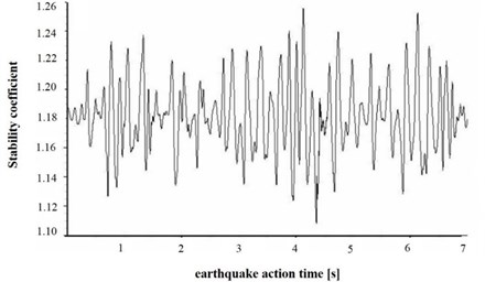
Fig. 9Probability distribution of slope stability coefficient
3.4. Dynamic strength reduction method
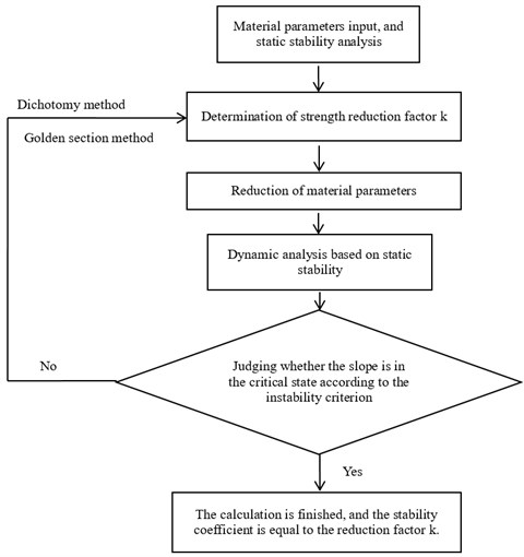
The static strength reduction method is intended to reduce the shear strength parameters of slope and into and respectively and then perform static analysis. When the slope reaches the limit equilibrium state under a certain reduction factor “”, the value of “”represents the stability coefficient of the slope [24]. Based on the principle of the static strength reduction method, the dynamic strength reduction method applies this kind of strength reduction theory to the dynamic stability analysis, and its analysis process is shown in Fig. 10.
Through the field investigation, it can be found that the failure of the slope under an earthquake is the composite failure of tension and shear. Therefore, it is necessary to consider the shear failure and tensile failure of the slope in the seismic stability analysis [25]. The following reduction formula is used in this paper.
where, ,, and are respectively the cohesion, internal friction angle and tensile strength of slope rock in the initial state; , , and are the cohesion, internal friction angle and tensile strength of slope rock after reduction; is the reduction coefficient.
The dynamic strength reduction method is essentially a kind of a search algorithm, which determines the critical failure state of slope through constantly adjusting the reduction factor. Therefore, judging the instability state of slope is the key problem in the dynamic strength reduction method. Under the static condition, the judgment standard of the slope instability mainly adopts the following three categories: (a) judging according to the stress distribution of the slope, for example, whether there is a perforated plastic zone in the slope body; (b) judging according to the deformation characteristics of the slope, such as the displacement mutation of the key slope point; (c) judging according to whether the numerical calculation is convergent. The judgment method of perforated plastic zone in the slope body is more applied to the calculation of soil slope. Besides, there is no concept of convergence for the dynamic strength reduction method. Therefore, the slope deformation characteristics are used as the basis for a judging criterion in the dynamic stability of bedding rock slope.
Fig. 10Calculation flow chart of dynamic strength reduction method
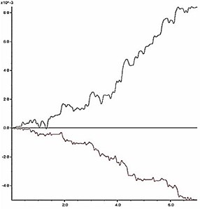
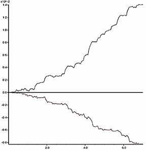
The slope shoulder is chosen as the key point to analyze the dynamic stability of model slope, and the curve characteristics of the horizontal and vertical deformation of the key point are chosen as the judging criterion. During an earthquake, the horizontal and vertical deformation of the slope shoulder under different reduction coefficients are shown in Fig. 11. According to the results in Fig. 11, the relation between the permanent deformation of the slope and the reduction coefficient is obtained as shown in Fig. 12.
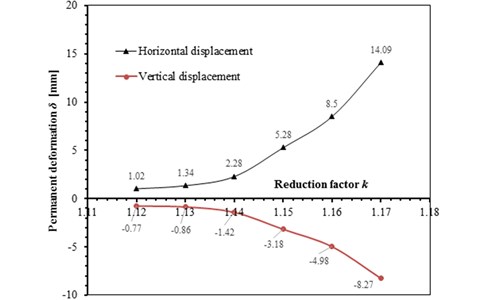
The deformation characteristic of the key point is the basis for judgment of slope instability. According to Fig. 11 and Fig. 12, two aspects should be considered when judging the slope instability condition: a) shape of deformation time-history curve, and b) increase amplitude of the cumulative permanent deformation. When the reduction coefficient is small, and the slope is in stable condition, obvious sharp oscillation and fluctuation can be seen from the deformation curve, and the deformation has a trend of convergence after the earthquake action. Meanwhile, the permanent deformation shows a small increase with low amplitude. As the reduction coefficient increases, the slope gradually becomes unstable. At this time, the deformation curve gradually becomes smooth with fewer sharp oscillations and shows a significant growth trend during the dynamic action. Moreover, the permanent deformation shows a significant increase with a high amplitude.
As shown in Fig. 11, when 1.14, time history curves of deformation of the key point have a trend of convergence after the earthquake action; when , the shape of time history curve has a larger change, which has no trend of convergence. As shown in Fig. 12, when , the change rate of the permanent deformation with is very low; when , the change rate of the permanent deformation with k shows a trend of rapid growth. According to the results in Fig. 11 and Fig. 12, when the reduction coefficient is 1.14, the model slope is in the state of critical instability. Therefore, the reduction coefficient can be considered as the dynamic stability coefficient of the model slope.
Fig. 11Horizontal and vertical deformation time-history curves of key point under different reduction coefficients
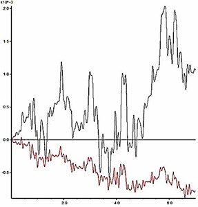
a) 1.12
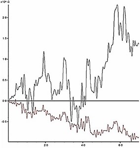
b) 1.13
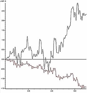
c) 1.14
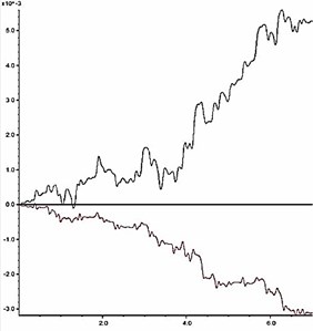
d) 1.15
e) 1.16
f) 1.17
3.5. Comparison of three methods
For the same model slope, the stability coefficient calculated by the pseudo-static method is 1.24, however, the result of dynamic strength reduction method is 1.14, which is close to the calculation results of 1.142 when the failure probability is 0.05 by the dynamic time-history method. Obviously, the result of the pseudo static method is larger than that of the latter two methods. When the dynamic time-history method is used, the time-history curve of stability coefficient needs to be further processed. However, there is still no unified processing method at present. In this paper, the probability and statistics method is adopted to process the time-history data, which links the stability evaluation index with the failure probability, but there is still no uniform acceptable failure probability. When using the dynamic strength reduction method, there are two main restriction factors, one is how to judge the critical state, and the other one is the dynamic response distortion. But for the bedding rock slope, the failure occurs mainly along the structure plane in the slope, and the critical state of slope can be well judged by the deformation characteristics of the key points on the sliding body. Besides, the dynamic response distortion of the slope is limited and acceptable by only reducing the strength parameters of the slope bedding surface. Therefore, the dynamic strength reduction method is more suitable for the dynamic stability analysis of bedding rock slope. Based on this, the dynamic strength reduction method is used to analyze influencing factors of dynamic stability of bedding rock slope in this paper.
Fig. 12Relationship between reduction coefficient k and permanent deformation δ
4. Influencing factors of slope dynamic stability
4.1. Numerical analysis model
The geometric dimensions and boundary conditions of the model slope are shown in Fig. 13.
Fig. 13Geometric dimensions and boundary conditions of model slope
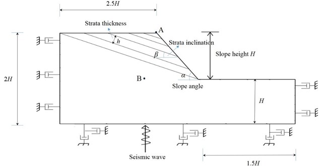
In Fig. 13, represents the slope angle, represents the slope height, represents the strata inclination, and represents the strata thickness. In order to reduce the influence of boundary conditions, the geometric size of the model slope is set as follows: the horizontal length at the top and foot of the slope is respectively 2.5 and , and the total height between the upper and lower bounds is .
The rock material in the model is in line with the ideal elastic-plastic constitutive model and is subject to the Mohr-Coulomb strength criterion, and the contact element is used to simulate the structure plane. Physical and mechanical parameters of the slope rock and structure plane are shown in Table 5 and Table 6 respectively.
Table 5Physical and mechanical parameters of slope rock
Cohesion / MPa | Friction angle / (°) | Shear modulus / GPa | Bulk modulus / GPa | Density / kg·m-3 | Tensile strength / MPa | Damping ratio | |
Metamorphic rock | 1.0 | 38 | 4.167 | 5.556 | 2500 | 0.7 | 0.048 |
Table 6Mechanical parameters of structural plane
Normal stiffness / (GPa·m-1) | Tangential stiffness / (GPa·m-1) | Friction angle / (°) | Cohesion / kPa | Tensile strength / kPa |
12.4 | 8.6 | 30 | 30 | 10 |
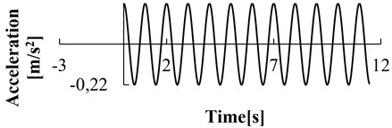
The boundary condition is set to be the viscous boundary, and the local damping coefficient is 0.15. The cosine shear wave was chosen as the input wave of dynamic load, as shown in Fig. 14, the time-history curve of the acceleration is in accordance with the following formula, i.e. , where, 0.22m/s2, is the frequency. Due to the viscous boundary condition, the input of the dynamic load needs to transform acceleration time-history data into stress time-history data.
Fig. 14Acceleration time-history curve of seismic wave (λ= 0.22 m/s2, f= 3 Hz)
4.2. Judgment of critical state and sliding surface
According to the foregoing analysis, through the deformation characteristics of the key points in bedding rock slope, the judgment problem of the critical state can be well solved in order to determine the critical state of the slope more accurately. In this example, take the convergence of time history curve of the horizontal displacement difference between the point A of slope shoulder and point B in the bedrock in Fig. 13 as the basis of the judgment. In Fig. 13, the failure mode of the slope is mainly along the bedding plane. When the slope is instable, the displacement of the upper and lower strata of the sliding surface will appear obvious mutation. Therefore, the potential slip surface can be determined according to the horizontal displacement contour of the slope.
4.3. Analysis results of influencing factors
4.3.1. Dynamic load frequency
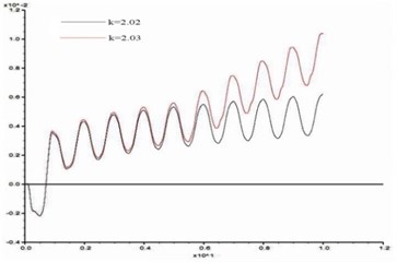
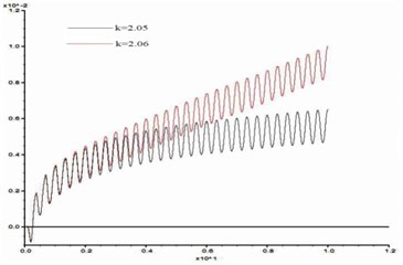
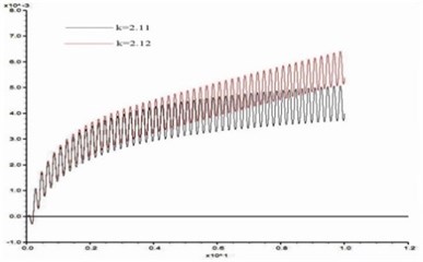
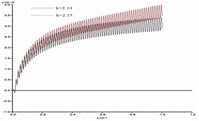
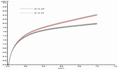
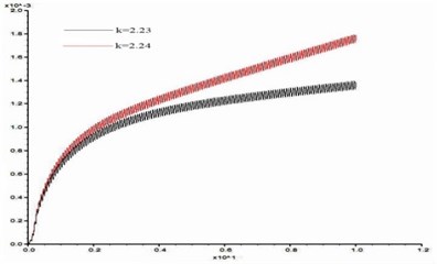
In order to study the influence of dynamic load frequency on the stability of bedding rock slope, six groups of cosine shear waves with frequency 1 Hz, 3 Hz, 5 Hz, 7 Hz, 10 Hz, 15 Hz respectively are applied on the model slope ( 100 m, 60°, 10 m, 15°), and the displacement difference curves between point A and point B were obtained when the slope was in the critical state. These time-history curves are shown in Fig. 15.
Fig. 15Time history curves of horizontal displacement difference between point A and B in critical state (α= 60°, H= 100, β= 15°, h= 10 m)
a) 1 Hz
b) 3 Hz
c) 5 Hz
d) 7 Hz
e) 10 Hz
f) 15 Hz
From Fig. 15, the stability coefficients of the slope under six groups of frequencies are 2.02, 2.05, 2.11, 2.14, 2.20 and 2.23 respectively. Thus, the relation between the slope stability and the dynamic load frequency can be obtained as shown in Fig. 16. According to Fig. 16, the dynamic stability of the slope increases with the frequency increase from 1 Hz to 3 Hz, the increase rate of stability coefficient is relatively slow; in the range of 3 Hz-10 Hz, the stability coefficient is approximately linear up; from 10 Hz-15 Hz, the rising trend of stability coefficient gradually tends to be gentle. This law shows that the dynamic stability of the slope is greatly influenced by a middle and low frequency part of the dynamic load but less influenced by its high frequency part.
4.3.2. Slope angle
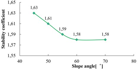
Take five groups of model slope ( 100 m, 20°, 10 m, 3 Hz) with slope angle of 45°, 50°, 55°, 60°, 70° respectively for a dynamic numerical calculation. Through the aforementioned method, the relation curve between the slope angle and the dynamic stability coefficient of the slope is shown in Fig. 17.
As shown in Fig. 17, the dynamic stability coefficient of the slope is almost linearly decreased with the slope angle increase when the slope angle is within the range of 45°-55°; the stability coefficient of the slope gradually tends to be stable when the slope angle is within the range of 55°-70°.
Fig. 16Relation between stability coefficient and frequency of dynamic load (α= 60°, H= 100 m, β= 15°, h= 10 m)
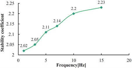
Fig. 17Relation between stability coefficient and slope angle (H= 100 m, β= 20°, h= 10 m, f= 3 Hz)
4.3.3. Slope height
Take five groups of model slope ( 60°, 20°, 10 m, 3 Hz) with the slope height 60 m, 100 m, 150 m, 200 m, 300 m respectively for a dynamic numerical calculation. The relation curve between the slope height and the dynamic stability coefficient of the slope is shown in Fig. 18. From Fig. 18, the dynamic stability coefficient gradually decreases with the increase of the slope height. In the range of 60-200 m, the stability coefficient changes rapidly with slope height, which shows that slope stability is sensitive to the influence of slope height in this range; within the range of 200-300 m, the stability of the slope is less influenced by slope height.
4.3.4. Strata inclination
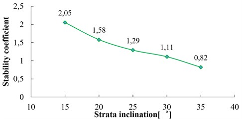
Take five groups of model slope ( 60°, 20°, 10 m, 3 Hz) with the strata inclination 15°, 20°, 25°, 30°, 35° respectively for a dynamic numerical calculation. The relation curve between the strata inclination and the dynamic stability coefficient of the slope is shown in Fig. 19. From Fig. 19, the dynamic stability coefficient of the slope decreases obviously with the increase of the strata inclination, and the variation amplitudes are relatively large. The slope stability coefficient decreases by 60 % when the strata inclination increases from 15° to 35°. Obviously, the strata inclination has a direct and important influence on the stability of the bedding rock slope.
Fig. 18Relation between stability coefficient and slope height (α= 60°, β= 20°, h= 10 m, f= 3 Hz)
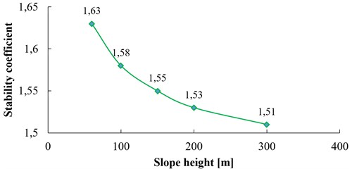
Fig. 19Relation between stability coefficient and strata inclination (α= 60°, H= 100 m, h= 10 m, f= 3 Hz)
4.3.5. Strata thickness
Take four groups of model slope ( 60°, 100 m, 25°, 3 Hz) with the strata thickness 5 m, 8 m, 10 m, 15 m respectively for a dynamic numerical calculation. The relation curve between the strata thickness and the dynamic stability coefficient of the slope is shown in Fig. 20.
Fig. 20Relation between stability coefficient and strata thickness (α= 60°, H= 100 m, β= 25°, f= 3 Hz)
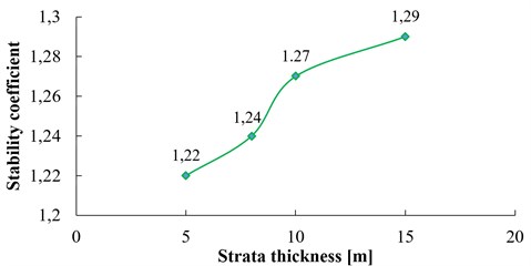
As it can be seen in Fig. 20, when the strata thickness is below 10 m, the dynamic stability of the slope increases with the increase of strata thickness, however, the stability coefficient basically tends to be stable when the strata thickness exceeds 10 m, and the dynamic stability of slope will almost not be affected by strata thickness.
5. Discussion
5.1. Mechanism of five factors above influencing on slope dynamic stability
5.1.1. Dynamic load frequency
The dynamic stability of slope is not only related to the dynamic load magnitude, but also can be greatly influenced by the dynamic characteristics of the slope itself, such as the natural frequency, damping ratio and so on. Under the condition of the same duration and amplitude, when the frequency of dynamic load is close to the natural frequency of the slope, the slope will get more unstable.
In order to get the natural frequency of the model slope as shown in Fig. 13, the dynamic load shown in Fig. 6 was applied at the bottom of the model, and the acceleration variation of the slope shoulder in the duration of dynamic action was monitored, so the acceleration curve of slope shoulder will be obtained. The distribution of the acceleration signal in the frequency domain is obtained through the Fourier transform of the acceleration curve, as shown in Fig. 21.
Fig. 21Fourier transform amplitude spectrum of acceleration response in slope shoulder
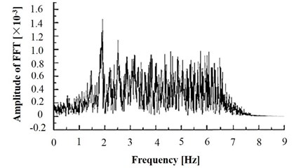
As it can be seen from Fig. 21, the maximum intensity responding of the acceleration is concentrated in the frequency band of 1.5 Hz-2.5 Hz. Thus, the natural frequency of the model is about 2 Hz. In Fig. 16, due to the frequency of 1 Hz, 3 Hz are close to the natural frequency of slope, the slope dynamic stability is the worst under the load with these two frequencies. As the load frequency increases, the stability coefficient of slope increases correspondingly.
5.1.2. Slope angle
Limit equilibrium theory is adopted in this section to analyze the effect of slope angle on slope dynamic stability, with schematic diagrams shown in Fig. 22.
Fig. 22Calculation schematic diagram of slope stability coefficient with different slope angles
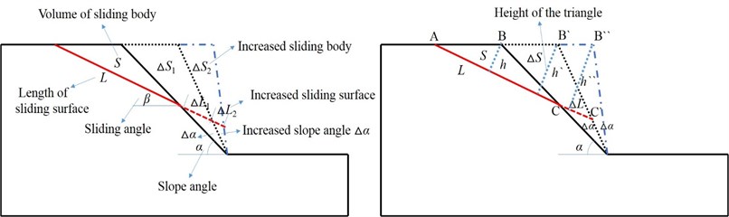
The following calculation of slope stability only takes the influence of slope gravity and horizontal seismic force into account. Based on limit equilibrium theory and Fig. 22, the equation for calculating slope stability coefficient is obtained as follows:
where is the density of sliding body, is the sliding volume of unit thickness, is the increased volume of sliding body, is slip length, is the increased slip length, is the horizontal seismic acceleration exerting on the center of slip gravity, is the cohesive strength of sliding surface, and is the friction angle of sliding surface. When the initial condition of the slope is determined, , , , , , are all fixed values. Therefore, the Eq. (9) can be rewritten as the following type:
In Eq. (10), , are both constants:
As shown in Fig. 22, the area of the triangle AB'C' is:
where is the height of the triangle AB'C, as shown in Fig. 22. Take Eq. (11) into the Eq. (10), the following equation can be obtained as follows:
According to Eq. (12) and Fig. 22, with the increase of slope angle, the stability coefficient of the slope will decrease continuously due to the increase of . However, when the slope angle is increased by the same angle of , the length of B'B" is less than that of BB' in Fig. 22, which indicates the descent speed of slope stability coefficient will be significantly reduced with the increase of slope angle. In Fig. 17, when the slope angle increases from 45° to 55°, the slope stability coefficient will decrease from 1.63 to 1.59. When the slope angle increases from 55° to 70°, the slope stability coefficient remains almost unchanged (from 1.59 to 1.58), which is consistent with the laws analyzed above.
5.1.3. Slope height
The dynamic stability of slope is closely related to the dynamic slope response According to the related research, the dynamic slope response has the “elevation effect”, that is, as the slope height increases, the dynamic slope response will get more intense. In order to study the influence of slope height on the dynamic response, the dynamic response of three slopes with the height of 60 m, 150 m, 300 m respectively are monitored, and the results are shown in Fig. 23. In Fig. 23, the PGA value is the ratio between the peak value of acceleration at corresponding monitoring points (1, 2, 3, 4) and that at the slope toe (point 0), which represents the amplification coefficient of acceleration (that is, the dynamic response degree) of each measuring point. From Fig. 23, as the slope height increases, the PGA of each measuring point increases continuously, which means the dynamic response of slope becomes more intense. When slope height increases from 60 m to 150 m, the increase amplitude of PGA is significantly higher than that of slope height increasing from 150 m to 300 m. In Fig. 18, when slope height increases from 60 m to 150 m, the stability coefficient of the slope is decreased by 4.9 %. But when slope height increases from 150 m to 300 m, the stability coefficient is only decreased by 2.6 %, which is consistent with the law of dynamic slope response mentioned above.
In addition, according to the statistics of rock landslides caused by Wenchuan earthquake, the relation between the number of landslides and slope height is shown in Fig. 24. From Fig. 24, we can see that the height of slope instability is mainly concentrated within range of 200 m-300 m above the valley, which is instructive to further study the influence of slope height on the slope dynamic stability.
Fig. 23Dynamic response characteristics of slope with different heights
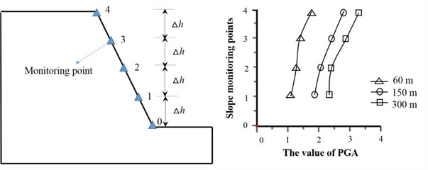
Fig. 24Relation between the number of landslides and the slope height (based on the statistics of Wenchuan earthquake) [18]
![Relation between the number of landslides and the slope height (based on the statistics of Wenchuan earthquake) [18]](https://static-01.extrica.com/articles/17210/17210-img40.jpg)
5.1.4. Strata inclination
In numerical simulation in Section 4, the strata inclination varies from 15° to 45°, which are all less than the slope angle (60°). Thus, the bedding surfaces will be exposed in the slope surface. Considering failure modes of the slope, the influence of strata inclination on slope stability can be analyzed based on limit equilibrium theory. According to Fig. 7, when substituting Eqs. (2), (3) into Eq. (1), the relation between slope stability coefficient and strata inclination can be obtained as follows (without considering the influence of groundwater):
As can be seen in Eq. (13), with the increase of strata inclination, the sliding force of the sliding surface increases, and the anti-sliding force decreases, which leads to a significant reduction in slope stability. In Fig. 19, the slope stability coefficient almost decreases linearly with the increase of strata inclination, and there is no convergence trend, which is consistent with the results of Eq. (13) calculated by the limit equilibrium theory.
5.1.5. Strata thickness
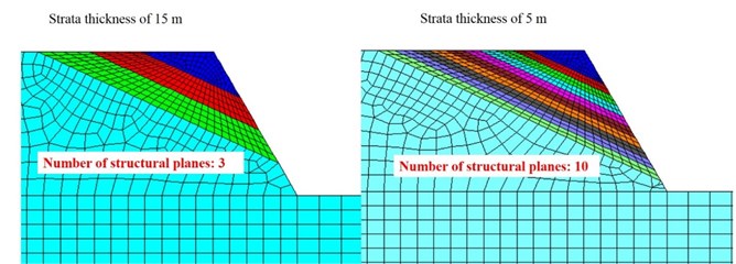
The bedding surfaces are discontinuous structure planes in rock slope. When the vibration stress wave spreads to these planes, a complex wave field will be formed due to the action of reflection and refraction (as shown in Fig. 26), which leads to the slope acted by repeated tension and compression forces, and finally leads to the damage of the internal structure. The above phenomenon is the “bedding surface effect” of slope dynamic response. In numerical simulation in Section 4, when the slope size and shape is determined, there will be more bedding surfaces with lower strata thickness, on the contrary, fewer bedding surfaces with higher strata thickness. As shown in Fig. 26, when the strata thickness is 15 m, the number of structural planes is 3, and when strata thickness decreases to 5 m, the number of structural planes in the slope increases to 10, which leads to the significant refraction and reflection of the seismic wave in the slope. The slope stability will be significantly reduced under this complex wave field.
Fig. 25Refraction and reflection of seismic waves in structural plane
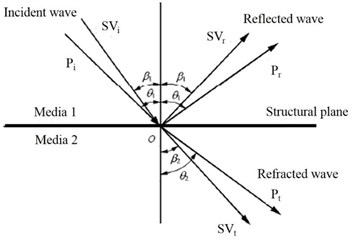
Fig. 26Number of structural planes with different strata thickness
5.2. Differences in results of stability analysis between the dynamic and static conditions
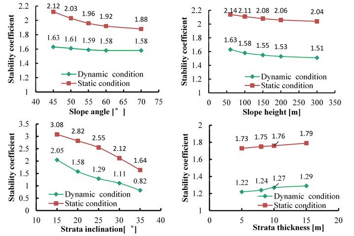
The influence of slope height, slope angle, strata inclination and strata thickness on the dynamic stability has been analyzed in Section 4. However, the static stability of the slope is also greatly affected by these parameters. Based on the strength reduction method under static condition, the variation of static stability coefficient with the change of four parameters above was obtained, and the calculation results were compared with the results under the dynamic condition, which were shown in Fig. 27.
As can be seen in Fig. 27, the variation trend of stability coefficient under static and dynamic conditions is consistent, and the slope static stability of is obviously higher than the dynamic stability. Under static conditions, the strata inclination is also the most sensitive influencing factor. It is worth noting that when the slope height increases from 60 m to 300 m, the stability coefficient decreases 4.7 % in static condition, and decreases 7.4 % in dynamic condition; when strata thickness decreases from 15 m to 5 m, the stability coefficient decreases 3.4 % in static condition, and decreases 5.4 % in dynamic condition. It can be seen that the slope dynamic response has the “elevation effect” and “bedding surface effect” in the dynamic condition, which makes the slope height and strata thickness have a greater influence on the slope stability.
Fig. 27Comparison of slope stability coefficient under dynamic and static conditions
5.3. Failure mode of the model slope in numerical simulation
The bedding planes are exposed both in the top and surface of the slope in Section 4, it can be judged that the failure mode of slope will be the overall slip along breakthrough bedding planes. In addition, due to the acted dynamic load is small (with peak acceleration of 0.22 m/s2), the slope is difficult to form a tension crack at trailing edge, which is induced by strong earthquake, such as the Wenchuan earthquake. For there are several penetrating bedding planes in model slope, it’s necessary to study which bedding plane (shallow or deep) will be the sliding surface, especially when the geometric size of slope (slope angle, slope height and strata inclination) is changed.
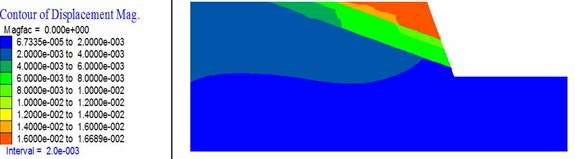
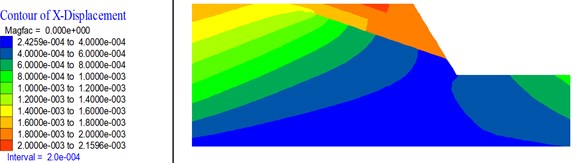
Fig. 28, Fig. 29, and Fig. 30 respectively show the horizontal displacement nephogram of slope in critical state of instability with different slope angle (45°, 70°), slope height (60 m, 300 m), and strata inclination (15°, 35°). As shown in Fig. 28, when the slope angle is gentle, the whole sliding of slope will occur along the deep plane. When the slope angle is relatively steep, there are two distinct sliding surface in the slope and slope instability is more likely to occur along the shallow plane. As shown in Fig. 29, when the slope height is small, integral slipping of the slope will occur along the deep plane. When the slope height increases, partial sliding instability is more likely to occur along the shallow plane. As shown in Fig. 30, when the strata inclination is gentle, there are several sliding surfaces and the deformation of the sliding body above the shallow sliding surface is larger. With the increase of strata inclination, the whole sliding instability is more likely to occur along the deep plane.
Fig. 28Horizontal displacement nephogram of the slope with different slope angle
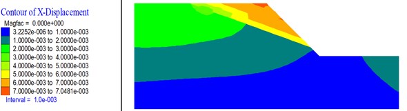
a) 45°
b) 70°
Fig. 29Horizontal displacement nephogram of the slope with different slope height
a)60 m
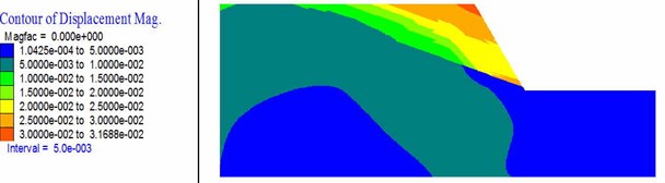
b)300 m
Fig. 30Horizontal displacement nephogram of the slope with different strata inclination
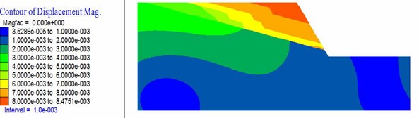
a) 15°
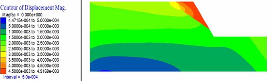
b) 35°
6. Conclusions
Based on the summary of typical failure modes of the bedding rock slope and differences in failure mode between dynamic and static conditions, two numerical calculation models of the bedding rock slope are established by using FLAC3D. A numerical analysis of three evaluation methods for the slope dynamic stability and of five factors influencing the stability is carried out respectively, and the following conclusions are obtained in this paper:
1) For the same example slope, the slope stability coefficient calculated by the pseudo static method is larger than that obtained by the latter two methods. When the dynamic time-history method is adopted, it is necessary to process further the stability time-history curve to get an evaluation index. However, there is still no unified processing method at present. In this paper, the probability statistical method is used to process the stability time-history curve. Although the stability evaluation index related to the failure probability can be gained, there is still no unified acceptable failure probability.
2) For the bedding rock slope, the failure occurs mainly along bedding surface in the slope, and the critical state of slope can be well judged by the deformation characteristics of the key points in the sliding body. Besides, the dynamic response distortion of the slope is limited and acceptable by only reducing the strength parameters of bedding surface in the slope. Therefore, the dynamic strength reduction method is more suitable for the dynamic stability analysis of bedding rock slope.
3) The dynamic stability of slope becomes worse when the load frequency is close to the natural frequency of slope. For the model slope in this paper, the dynamic stability of the slope increases with the increase of dynamic load frequency. Within the range of 3 Hz-10 Hz, the stability coefficient approximately increases in linear and within 10 Hz-15 Hz, the rising trend of stability coefficient gradually tends to be gentle. Obviously, the dynamic stability of the slope is greatly influenced by the middle and low frequency part of dynamic load but less influenced by its high frequency part.
4) Due to the “elevation effect” and “bedding surface effect” in the dynamic response of slope, the slope stability decreases with the increase of slope height and the reduction of strata thickness. However, the influence of these two parameters has a critical sensitivity value. For the example slope in this paper, when the slope height reaches 200 m, and the strata thickness reaches 10 m, the reduction of slope stability is no longer obvious with the increase of these two parameters.
5) Strata inclination has a direct and important influence on the dynamic stability of bedding rock slope. When the strata inclination increases from 15° to 35°, the slope stability coefficient can be reduced by 60 %, and it can be said that the strata inclination is the most sensitive parameter influencing slope stability. According to theoretical and numerical calculation results, the slope stability will decrease continuously with the increase of the slope angle. However, the descent speed of slope stability coefficient will be significantly reduced with the increase of the slope angle. For the model slope in this paper, when the slope angle reaches 55°, the reduction of slope stability will be no longer obvious, which means the critical sensitivity value of slope angle is 55°.
References
-
Huang R. Engineering Geology for High Rock Slopes. Science Press, Beijing, China. 2012
-
Sun S., Sun H., Wang Y., Wei J., Liu J., Kanungo D. P. Effect of the combination characteristics of rock structural plane on the stability of a rock-mass slope. Bulletin of Engineering Geology and the Environment, Vol. 73, Issue 4, 2014, p. 987-895.
-
Fan G., Zhang J., Fu X. Dynamic response differences between bedding and count-tilt rock slopes with siltized intercalation. Chinese Journal of Geotechnical Engineering, Vol. 37, Issue 4, 2015, p. 692-699.
-
Fan G., Zhang J., Fu X., Du L., Liu F. Large-scale shaking table test on dynamic response of bedding rock slopes with silt intercalation. Chinese Journal of Rock Mechanics and Engineering, Vol. 34, Issue 9, 2015, p. 1750-1757.
-
Xu Q., Liu H., Zou W., Fan X., Chen J. Large-scale shaking table test study of acceleration dynamic responses characteristics of slopes. Chinese Journal of Rock Mechanics and Engineering, Vol. 29, Issue 12, 2010, p. 2420-2428.
-
Hatzor Y. H., Arzi A. A., Zaslavsky Y., Shapira A. Dynamic stability analysis of jointed rock slopes using the DDA method: King Herod’s Palace, Masada, Israel. International Journal of Rock Mechanics and Mining Sciences, Vol. 41, Issue 5, 2004, p. 813-832.
-
Latha G. M., Garaga A. Seismic stability analysis of a Himalayan rock slope. Rock Mechanics and Rock Engineering, Vol. 43, Issue 6, 2010, p. 831-843.
-
Li X., Tang H., Hu W. Effect of bedding plane parameters on dynamic failure process of sliding rock slopes. Chinese Journal of Geotechnical Engineering, Vol. 36, Issue 3, 2014, p. 466-473.
-
Scholtes L., Donze F. Modelling progressive failure in fractured rock masses using a 3D discrete element method. International Journal of Rock Mechanics and Mining Sciences, Vol. 52, 2012, p. 18-30.
-
Newmark N. M. Effect of earthquakes on dams and embankments. Geotechnique, Vol. 15, Issue 2, 1965, p. 139-160.
-
AI-Homo A. S., Tahtamoni W. W. Reliability analysis of three-dimensional dynamic slope stability and earthquake-induced permanent displacement. Soil Dynamics and Earthquake Engineering, Vol. 19, Issue 2, 2000, p. 91-114.
-
Erfani Joorabchi A., Liang R. Y., Li L., et al. Yield acceleration and permanent displacement of a slope reinforced with a row of drilled shafts. Soil Dynamics and Earthquake Engineering, Vol. 57, 2014, p. 68-77.
-
Yang X. L. Seismic bearing capacity of a strip footing on rock slopes. Canadian Geotechnical Journal, Vol. 46, Issue 8, 2009, p. 943-954.
-
Wu Y., Liu D., Song Q., Ou Y. Reliability analysis of slope dynamic stability based on strength reduction FEM. Rock and Soil Mechanics, Vol. 34, Issue 7, 2013, p. 2084-2090.
-
Harp E. L., Hartzell S. H., Jibson R. W., Ramirez-Guzman L., Schmitt R. G. Relation of landslides triggered by the Kiholo Bay Earthquake to modeled ground motion. Bulletin of the Seismological Society of America, Vol. 104, Issue 5, 2014, p. 2529-2540.
-
Huang R., Zhang W., Pei X. Engineering geological study on Daguangbao landslide. Journal of Engineering Geology, Vol. 22, Issue 4, 2014, p. 557-585.
-
Huang R., Li G., Ju N. Shaking table test on strong earthquake response of stratified rock slopes. Chinese Journal of Rock Mechanics and Engineering, Vol. 32, Issue 5, 2013, p. 865-875.
-
Li G. Failure Mechanism of Strati-Form Rock Slope under Strong Earthquake. Chengdu University of Technology, Ph.D. Thesis, Chengdu, China, 2012.
-
Liu J., Li J., Zhang Y., Qu J., Li J., Li Y. Stability analysis of Dagangshan dam abutment slope under earthquake based on pseudo-static method. Chinese Journal of Rock Mechanics and Engineering, Vol. 28, Issue 8, 2009, p. 1562-1570.
-
Liu H., Fei K., Gao Y. Time history analysis method of slope seismic stability. Rock and Soil Mechanics, Vol. 24, Issue 4, 2003, p. 556-560.
-
Zhang B., Chen H., Du X., Zhang Y. Arch dam abutment asiesmatic stability analysis. Journal of Hydraulic Engineering, Vol. 11, 2000, p. 55-59.
-
Zheng Y., Ye H., Huang R., Li A., Xu J. Study on the seismic stability analysis of a slope. Journal of Earthquake Engineering and Engineering Vibration, Vol. 30, Issue 2, 2010, p. 173-180.
-
Liu H., Tang L., Bo J., et al. New method for determining the seismic safety factor of a rock slope. Journal of Harbin Engineering University, Vol. 9, 2009, p. 1007-1011.
-
Matsui T., San K. Finite element slope stability analysis by shear strength reduction technique. Soils and Foundations, Vol. 32, Issue 1, 1992, p. 59-70.
-
Zheng Y., Den C., Tang X., et al. Development of finite element limiting analysis method and its application in geotechnical engineering. Engineering Sciences, Vol. 3, Issue 5, 2007, p. 10-36.
Cited by
About this article

The authors acknowledge the financial support provided by The National Natural Science Foundation of China (No. 41372356), 2015 Chongqing University Postgraduates’ Innovation Project (No. CYB15038) and The Fundamental Research Funds for the Central Universities (No. 106112014CDJZR200008).
Xinrong Liu set the framework of this paper, and provided funding for this research. Yongquan Liu wrote this paper, and completed most of revision tasks for this paper. Yuming Lu completed the fifth section “5 Discussion” of this paper and a few revision tasks. Xingwang Li established the numerical model of the slope in this paper. Peng Li completed the section “3.4 Dynamic Strength Reduction Method”.
