Abstract
The health state of a rolling bearing keeps changing from a normal state to a slight degradation state followed eventually by a severely degraded state. To make reasonable inspection and maintenance plans, it is necessary to estimate the degradation state and predict the lifetime of a running rolling bearing accurately and in a timely fashion. This paper presents a new method for rolling bearing degradation state estimation and lifetime prediction based on curve similarity recognition. Different from existing methods, this method employs a dynamic time warping algorithm to recognize the curve similarity of those extracted features of rolling bearings in different states of health, which can reflect the intrinsic state of the rolling bearing; it discretizes the bearing degradation state reasonably through curve similarity. Next, the curve similarity is used to train the degradation state estimation model and a support vector machine based lifetime prediction model. Finally, this paper conducts a case study for a rolling bearing with impact degradation and one with wear degradation, respectively. The experimental results indicate that the new proposed method is highly efficient in recognizing the bearing’s degradation state and predicting its lifetime.
1. Introduction
Rolling bearings are the most widely used component in rotary machinery, and their state of health is critical to all the equipment. However, rolling bearings’ lifetime is more scattered than other machine elements; i.e., some bearings might break down while their running time has not yet reached the designed lifetime, but some other bearings could still run normally while their running time far surpasses the designed lifetime. So, conducting real-time degradation state estimation and lifetime prediction for rolling bearings could not only avoid severe failure, but could also reduce the waste of resources.
However, there are many challenges that exist in recognizing the state of degradation and predicting the lifetime based on data driven by a rolling bearing. The most significant of these issues is figuring out how to extract appropriate features from bearing vibration signals. In recent years, many scholars have studied feature extraction methods used for degradation state estimation and lifetime prediction. Shao et al. and Pham used the root mean square and the kurtosis factor of the vibration signal to assess the performance degradation and predict a bearing’s remaining life [1, 2]. Wei et al. applied ensemble empirical mode decomposition to decompose bearing vibration signals to obtain the features used for a degradation state estimation [3]. Liao and Lee utilized wavelet packet decomposition and principal component analysis to extract features of bearing vibration signals [4]. Similarly, Huang et al. took three time-domain features and three frequency-domain features as degradation indexes and combined them with a self-organizing map and neural network to assess the performance and predict the lifetime of bearings [5]. Mahamad et al. used time and fit measurements of Weibull hazard rates by root mean square and the kurtosis as the input for an artificial neural network, which was applied to improve the accuracy of lifetime prediction [6]. Benkedjouh et al. first extracted the features from monitoring signals by wavelet packet decomposition and then reduced the dimensionality of the features by ISOMAP to predict the bearing lifetime [7]. Lu et al. utilized the selected chaotic characteristics of vibration signal for health assessment of a bearing by using self-organizing map (SOM) [8].
Generally, the predictions that use features extracted from the vibration signal can be divided into two types. One is to estimate the degradation state by features, based on dividing the degradation state across the whole bearing life time according to running time. This classification method ignores the physical laws of bearing degradation. The other is to directly use these features for lifetime prediction. However, the features of the vibration signals used in this type of estimate are relatively stable in the early stage of a bearing’s life, so the prediction error is relatively large.
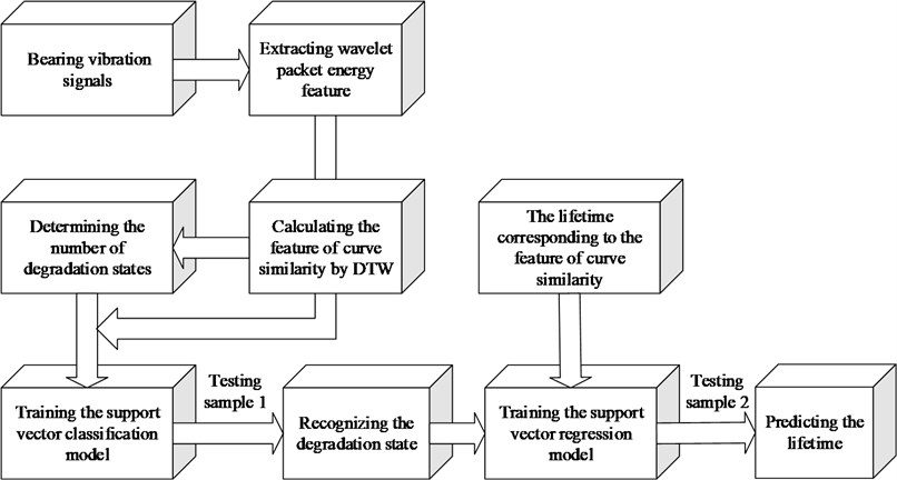
Little research has focused on using curve similarity of the extracted features to estimate the bearing degradation state and predict the bearing lifetime. In this paper, we present a new scheme to explore the laws of bearing degradation, as shown in Fig. 1. First, we use a dynamic time warping (DTW) algorithm to obtain the feature of a curve similar to the wavelet packet energy features that are extracted from the rolling bearings’ vibration signals at different health states based on wavelet packet decomposition (WPD). Next, the degradation state is discretized across the whole lifetime of the bearings according to the curve similarity. Next, the curve similarity is taken as a training sample to train a support vector machine (SVM) for the degradation state estimation model and lifetime prediction model. Finally, the vibration signals of rolling bearings with impact degradation and wear degradation are used to verify the effectiveness and practicability of the new method.
Fig. 1The overall flow diagram of the new scheme
2. Feature extraction
Wavelet packet decomposition (WPD) is a method of decomposing signals both in low-frequency and high-frequency ranges and has the ability to characterize local features in a time-frequency domain. Therefore, WPD is quite suitable for detecting transient anomalies in normal signals and has significant application value [9-11]. As for a given orthogonal scaling function, , and the wavelet function, , the two-scale relation equations are as follows:
where and are regarded as the filter coefficients of low-pass and high-pass filters, respectively. Next, the following recursion formula is defined to further extend the two-scale relation equations:
where and are still regarded as the filter coefficients. If 0, then and . Thus, the wavelet packets are a set of scaling functions and wavelet generating functions; i.e., a set of functions with a certain link.
WPD is a type of linear transformation and obeys the law of energy conservation. When decomposing the bearing vibration signal by WPD, the energy of the signal is also decomposed into different frequency bands, and the energy in each frequency band will change as the bearing degrades. Therefore, it is feasible to take the frequency band energy obtained by WPD as the feature to reflect the running state of bearings. The result of WPD expressed by energy is called the energy spectrum [12].
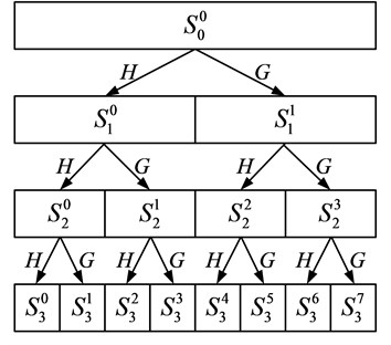
Taking a three-layer WPD of the original signal , as an example, is shown in Fig. 2; represents the low frequency component, and represents the high frequency component. The feature extraction method of wavelet packet energy spectrum is as follows:
1) Decompose vibration signal into three layers with WPD and obtain the coefficients of 8 sub-bands in third layer .
2) Reconstruct the signal of each sub-band by the WPD coefficients and represent as: (0, 1,..., 7). Then, the original signal .
3) Calculate the energy of the signal in each sub-band, and represent the energy corresponding to (0, 1,..., 7) as (0, 1,..., 7). Then:
where (0, 1,..., 7; 0, 1,..., ) is the amplitude of each discrete point in the reconstructed signal (0, 1,..., 7).
4) Construct the feature vector .
According to the energy spectrum of the bearing vibration signal obtained by wavelet packet decomposition, the running state of the bearing can be monitored.
3. Process of degradation state estimation and lifetime prediction
3.1. Calculating the curve similarity by DTW
Dynamic time warping (DTW) is a type of algorithm for matching patterns that are globally or locally extended, compressed and deformed. A DTW algorithm aims at realizing the similarity between measures and classifications of dynamic models. It was first used in the field of speech signal recognition as an effective similarity recognition tool; DTW algorithms have been widely used in many fields, such as fault diagnosis, biological gene sequencing, handwriting recognition, data mining, and so on. Next, the principle of the DTW algorithm is explained [13-15].
Fig. 2Schematic diagram of wavelet packet decomposition
There are two-time series that are assumed to be:
To calculate the similarity of the two sequences using a DTW algorithm, an -by- matrix is constructed. The value of the matrix element is equal to the Euclidean distance between the two points and . Then, the value is expressed as:
A combination of the continuous elements from matrix element (1, 1) to (, ) is called a warping path: . The square root of the sum of all the elements of each warping path is calculated, and determine the minimum value; that is the accumulated distance obtained by DTW algorithm. Next, the accumulated distance between and is defined as:
where , and is the length of , and . Additionally, there are some restrictions for the warping path in the DTW algorithm, including boundary constraints, continuity constraints and monotonicity constraints.
1) Boundary constraints:
The boundary constraints suggest that the starting point and stopping point of all the warping paths are the same because the sequence of the two-time series are not changed.
2) Continuity constraints. The continuity constraints aim at preventing overexpansion in the warping process. As for two continuous points in a warping path, such as and , the continuity constraints are expressed as:
3) Monotonicity constraints. For two continuous points in a warping path, such as and , the monotonicity constraints are expressed as:
From point (1, 1) to (, ), these two sequences, and , are matched and the distance of each point is gathered. The final accumulated distance is the exact similarity between sequence and . According to the three restrictions, the recursion formula of Eq. (9) could be expressed as follow:
3.2. Degradation state estimation and lifetime prediction based on SVM
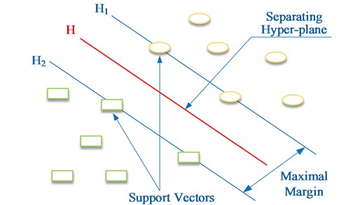
The support vector machine (SVM) was presented by Vapnik in 1995. SVM is a type of algorithm-based machine learning based on statistical learning theory and specifically targeted at small samples for training [16]. The basic principle of SVM is to map the input vectors into a high dimensional feature space and construct the optimum separating hyper-plane, to achieve classification. Take the classification of a two dimensional input space using linear SVM as an example, as shown in Fig. 3; the circles and squares represent two different classes of samples. is the classification curve. and are the curves parallel to the classification curve, and they include the samples that are the nearest to the classification curve for each class of samples. The distance between and is called the maximal margin. The samples that are the nearest to the classification curve are known as support vectors [17-20].
Fig. 3The principle of linear support vector machine in classification
Given a training sample set , each sample, , belongs to a classification of . Then, the classification curve can be expressed as , whereis a weight vector, and is a threshold. It has been proven that the maximal margin can be found by minimizing [16], subject to:
If the training set is not linearly separable, it needs to be converted into a high dimensional space. Assuming the transformation function and the kernel function is and , respectively, then:
As stated above, the optimal separating hyper-plane is as follows:
SVM is a type of binary classifier, and it is possible to solve multi-classification problems by combining multiple SVM classifiers. The SVM mentioned above is used as classifier and it is called a support vector classification (SVC). In this paper, the estimation of the degradation state of a rolling bearing could be regarded as a type of classification and is suitable for using SVC.
Furthermore, when applying the structural risk minimization principle of SVM to the design of regression, it is called “support vector regression” (SVR) [21, 22]. Given a training sample set, , and the linear regression problem in a high dimensional space to find the function:
where is a weight vector, is a threshold and is the mapping relationship. It has been proven that there are optimum solutions and making the regression model expression:
However, the mapping relationship, , from a low dimension to a high dimension is unknown in practical applications. The kernel function is introduced to complete the data mapping from low to high dimensions without knowing the mapping relationship, so Eq. (15) can be rewritten as:
Given a sample set of rolling bearing lifetime:
Part of the sample set is selected randomly as the training sample set, , and the training output as is recorded. Take the rest of the sample set as test sample and record the testing output as . Thus, the mean prediction error is defined as:
Therefore, taking the radial basis kernel function as an example, the training and parameter optimization of SVR gets the optimized parameters , which makes:
4. Case study
4.1. State estimation of the bearing with impact degradation
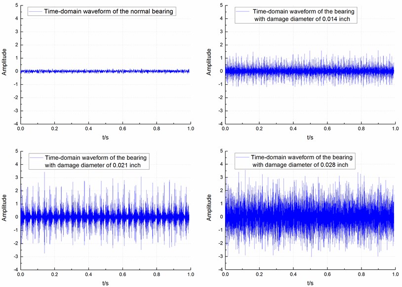
The vibration data of the bearing with impact degradation were generated are the Case Western Reserve University Bearing Data Center. The bearing model was 6205-2RS, and the sampling rate was 12 kHz. The damage diameter implanted into the bearings were 0.014 inch, 0.021 inch and 0.028 inch. The bearing load was 1 hp, and its rotational speed was 1772 rpm. When the sampling time of the vibration signal was 1 s, the time-domain waveform of the sampled signals of the bearings in the four types of states was generated, as shown in Fig. 4.
Fig. 4The time-domain waveform of the sampled signals of the bearings with four types of damage diameters
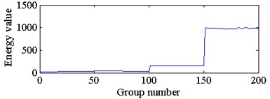
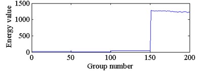
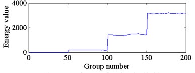
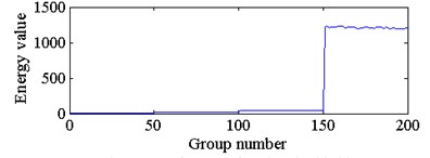
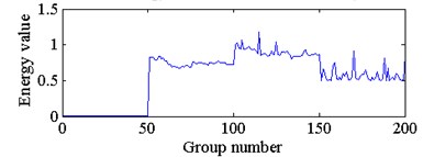
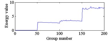
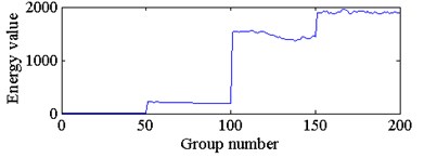
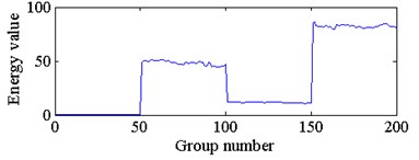
The energy spectrum of wavelet packet decomposition was used as the feature extracted from each sampled signal. This study decomposed each vibration signal into three layers with WPD, and obtained the energy spectrum of 8 sub bands in the third layer. The waveforms of the wavelet packet energies from four types of sampled signals are shown in Fig. 5. Where the sampling time of each group of sampled signal is 1 s, and the energy value of group 1-50, group 51-100, group 101-150 and group 151-200 belong to bearings with implanted damage diameters of 0 inch, 0.014 inch, 0.021 inch and 0.028 inch, respectively. The energy values from node 0 to node 7 correspond to the energy spectrum of the 8 frequency bands in the third layer from low frequency to high frequency.
With reference to Fig. 5, we can see that the wavelet packet energy in different frequency bands of the same sample signal have large differences. The wavelet packet energy of a bearing with the same damage diameter and the same frequency band has slight fluctuations. Based on the above theory of bearings with implanted damage diameters and the idea of curve similarity recognition, this paper adopts a DTW algorithm to obtain the similarity of the wavelet packet energy curves between the sampled signals of the bearing under the current state and normal state, as shown in Fig. 6.
Fig. 5The waveform of wavelet packet energy of four types of sampled signals
a) The energy feature of node 0 in third layer
b) The energy feature of node 1 in third layer
c) The energy feature of node 2 in third layer
d) The energy feature of node 3 in third layer
e) The energy feature of node 4 in third layer
f) The energy feature of node 5 in third layer
g) The energy feature of node 6 in third layer
h) The energy feature of node 7 in third layer
Fig. 6The curve similarity of the wavelet packet energy between the sampled signals of the bearing under current state and normal state
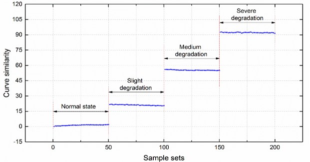
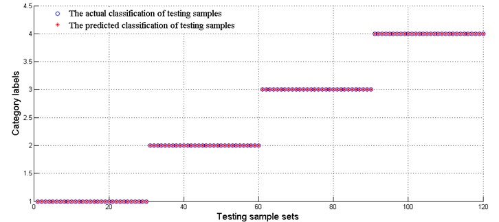
According to the curve similarity in Fig. 6, the degradation state of the bearings with four damage diameter sizes could clearly be divided into 4 stages. In this paper, the 4 stages are defined as a normal state, slight degradation state, medium degradation state and severe degradation state, and label the 4 degradation states as 1, 2, 3 and 4, respectively. Next, 20 groups of curve similarity of each degradation state were randomly selected as training samples for the SVR model, and the rest of the groups of curve similarity of each degradation state were used as testing samples. The training samples and testing samples could be considered as a curve similarity for the same type of bearings operating under the same working conditions. The comparison of actual degradation state and the recognized degradation state of the SVC model is shown in Fig. 7. The recognition accuracy of the testing samples is 100 %, which is equal to 120/120.
Fig. 7The actual and predicted classification of testing sample sets
The damage of the bearings with impact degradation used in this paper is artificially generated rather than being a natural bearing degradation by running the bearing. So, this paper only recognizes its degradation state, and does not predict its lifetime.
4.2. State estimation and lifetime prediction of the bearing with wear degradation
4.2.1. State estimation of the bearing with wear degradation
The vibration data of the bearings with wear degradation were generated by the NSF I/UCR Center on Intelligent Maintenance Systems (IMS). There were 350 groups of sampled signals during the whole life cycle of the bearing. The sampling time of each group of signals was 1s, and the sampling rate was 20 kHz. The vibration data were collected every 20 minutes by a NI DAQ Card 6062E.
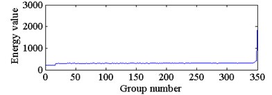
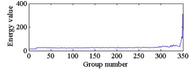
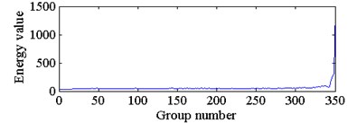
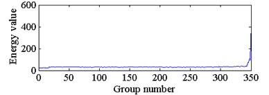
The energy spectrum of wavelet packet decomposition was used as the feature extracted from each group of sampled signals. This paper decomposes each group of vibration signal into three layers with WPD and obtain the energy spectrum of 8 sub bands in the third layer. The waveforms of wavelet packet energy feature from 350 groups of sampled signals are shown in Fig. 8. The energy values from node 0 to node 7 correspond to the energy spectrum of the 8 frequency bands in the third layer from low frequency to high frequency.
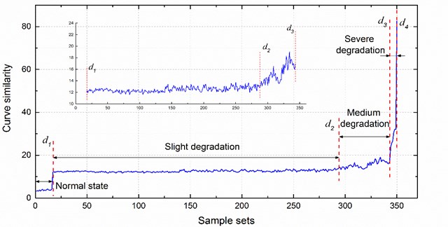
With reference to Fig. 8, we can see that the wavelet packet energy in different frequency bands of the same sampled signal have large differences in the full life cycle of the degraded bearing. Moreover, the wavelet packet energy in each frequency band will increase gradually with the increase of operation time of the bearing. When the bearing is about to fail, the wavelet packet energy increases rapidly. Based on the above principle of wear on bearing degradation and the idea of curve similarity recognition, this paper adopts a DTW algorithm to obtain the similarity of the wavelet packet energy curves between the sampled signals of the bearing under degradation states and normal state, as shown in Fig. 9.
According to the curve similarity in Fig. 9, the whole bearing lifetime could be divided into 4 stages, which is consistent with the general law of bearing degradation wear. In this paper, the 4 stages are defined as a normal state, slight degradation state, medium degradation state and severe degradation state. The dividing lines between the 4 states are labelled , , , and in Fig. 9 are the serial numbers, which are 15, 301, 343 and 350, respectively. In the normal state and sight degradation state, the fluctuation of the similarity curve of wavelet packet energy is very small. After entering the medium degradation state, the similarity curve increases gradually. If the similarity curve increases rapidly, it means the bearing is in a state of severe degradation.
Fig. 8The wavelet packet energy feature of 350 groups of sampled signals
a) The energy feature of node 0 in third layer
b) The energy feature of node 1 in third layer
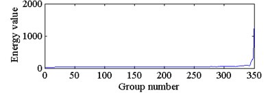
c) The energy feature of node 2 in third layer
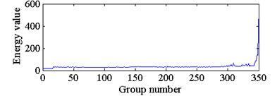
d) The energy feature of node 3 in third layer
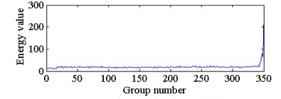
e) The energy feature of node 4 in third layer
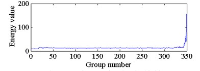
f) The energy feature of node 5 in third layer
g) The energy feature of node 6 in third layer
h) The energy feature of node 7 in third layer
Fig. 9The curve similarity of the wavelet packet energy between the sampled signals of the bearing under current degradation state and normal state
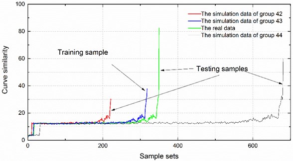
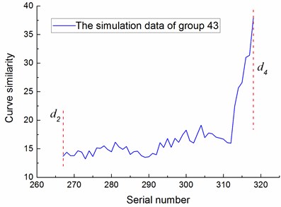
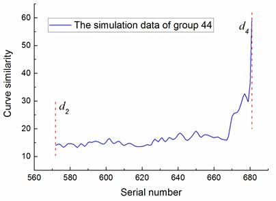
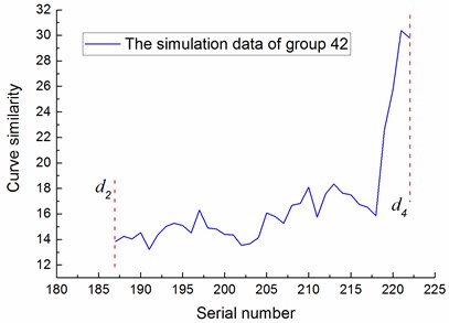
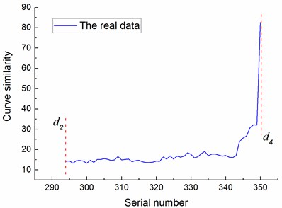
To train and test the SVC model to recognize the state of bearing degradation wear, this paper obtained 50 sets of simulation data by random selection and spline interpolation based on the real curve similarity, as shown in Fig. 10. Then, we labeled the 4 degradation states as 1, 2, 3 and 4, and selected the set of 43 of simulation data as the training sample for the SVC model. In addition, the real curve similarity was selected, and set 42 and 44 of simulation data were chosen as the testing samples of the SVC model, as shown in Fig. 11. The training sample and testing samples could be considered as the curve similarity of the same type of bearings operating under the same working condition. The comparison of actual degradation state and the recognized degradation state from the SVC model is shown in Fig. 12.
Fig. 10The real sample and simulation samples
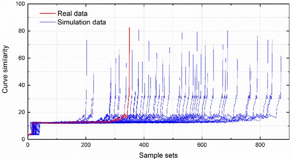
Fig. 11Training sample and testing samples of SVC model
Accurate degradation state estimation of a rolling bearing is the premise of predicting its lifetime accurately. The recognition accuracy of the simulation data of set 44 is 98.091 %, which is equal to 668/681. When the recognized bearing states are all at medium degradation state three consecutive times, the bearing is considered to have entered the medium degradation state. According to this rule, the simulation data of set 44 is in the third state after the group of 572, as shown in Fig. 12. Similarly, the recognition accuracy of the simulation data of set 42 is 97.2973 %, which is equal to 216/222. AT this set of simulation data is in third state after the group of 187. The recognition accuracy of the real sample is 98 %, which is equal to 343/350; the real sample is in third state after the group of 294.
4.2.2. Lifetime prediction of the bearing with wear degradation
As analysis in Section 4.2.1, the whole life time of the bearing with wear degradation is divided into 4 degradation states. When the bearing is in normal state and slight degradation state, the curve similarity of its wavelet packet energy features has less fluctuation, which means the bearing operates stably, and it is unnecessary to predict its lifetime.
Fig. 12Comparison of actual degradation state and the recognized degradation state of testing samples
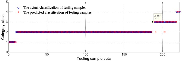
a) Comparison of actual degradation state and the recognized degradation state of set 42
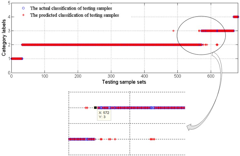
b) Comparison of actual degradation state and the recognized degradation state of set 44
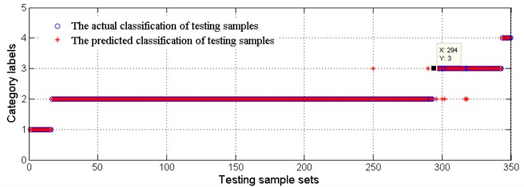
c) Comparison of actual degradation state and the recognized degradation state of real data
However, when the bearing is in the medium degradation state, its curve similarity increases gradually. If the curve similarity increases rapidly, it means that the bearing has entered the severe degradation state and it may fail in a short time. Therefore, to accurately know the state of the bearings in real time and make appropriate maintenance plans to prevent negative impacts on the whole system to be caused by sudden failure, it is necessary to predict the lifetime in a timely manner for bearings in a medium degradation state and severe degradation state.
To verify the feasibility of the lifetime prediction method proposed in this paper, the simulated curve similarity of set 43 after entering the medium degradation state and corresponding lifetime was taken as the training sample for the SVR model. Moreover, the real curve similarity and the simulated curve similarity of sets 42 and 44 after entering the medium degradation state were taken and the corresponding lifetime was the predicting samples for the SVR model. The curve similarity of wavelet packet energy of the training sample and predicting samples are shown in Fig. 13.
Fig. 13The curve similarity of wavelet packet energy of training sample and predicting samples
a) Training sample
b) Testing sample
c) Testing sample
d) Testing sample
The training sample was used to train the SVR model, and the trained SVR model was used to predict the lifetime of samples according to the curve similarity. Then, the predicted lifetime was compared with the actual lifetime of the three predicting samples, as shown in Fig. 14, using the calculation results of the formula to measure the accuracy of lifetime prediction, where MSE represents the mean square error, ActLtt represents the actual lifetime of the bearing at , and represents the predicted lifetime of the bearing at . In this study, lifetime is denoted by residual useful lifetime (RUL).
From Fig. 14, we can see that the trend of the predicted lifetime curve and actual lifetime curve are basically the same in this case study. The MSEs of the three predicting samples are 0.4712, 3.5164, and 0.5742, which are all in an acceptable range. Therefore, it can be concluded that the method proposed in this paper is able to predict maintenance need, reducing the outage time effectively and avoiding maintenance.
Fig. 14Comparison between the predicted and the actual values of the predicting samples
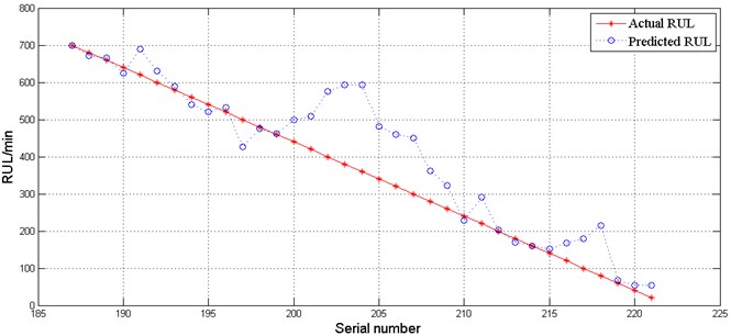
a) The actual lifetime and predicted lifetime of simulated data of set 42
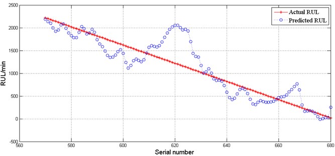
b) The actual lifetime and predicted lifetime of simulated data of set 44
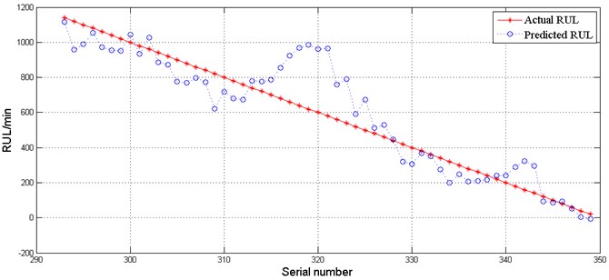
c) The actual lifetime and predicted lifetime of real data
5. Conclusions
In this paper, we proposed a method based on curve similarity recognition to estimate degradation state and predict lifetime, and conducted a case study using the vibration signals of rolling bearings with impact degradation and wear degradation. The results indicate that the new method is able to estimate bearing degradation state and predict its lifetime by extracting the wavelet packet energy features, calculating the curve similarity, and combining the SVC and SVR models. The main innovation of this paper is discretizing the degradation state of the whole bearing lifetime, and predicting the bearing’s lifetime by DTW algorithm calculated curve similarity.
The research in this paper focuses on the same type of bearings operating under the same working conditions. In the future, it would be meaningful to study the degradation state estimation and lifetime prediction for the same type of bearings operating under different working conditions with this method. In addition, improving the accuracy of the lifetime prediction is a possible direction for future research.
References
-
Shao Y., Nezu K. Prognosis of remaining bearing life using neural networks. Proceedings of the Institution of Mechanical Engineers, Part I: Journal of Systems and Control Engineering, Vol. 214, Issue 3, 2000, p. 217-230.
-
Pham H. T., Yang Nguyen B. S. T. T. Machine performance degradation assessment and remaining useful life prediction using proportional hazard model and support vector machine. Mechanical Systems and Signal Processing, Vol. 32, 2012, p. 320-330.
-
Wei Y., Wang M. Degradation state recognition of rolling bearing based on EEMD and SVM. Computer Integrated Manufacturing Systems, Vol. 9, 2015.
-
Liao L., Lee J. A novel method for machine performance degradation assessment based on fixed cycle features test. Journal of Sound and Vibration, Vol. 326, Issue 3, 2009, p. 894-908.
-
Huang R., Xi L., Li X., et al. Residual life predictions for ball bearings based on self-organizing map and back propagation neural network methods. Mechanical Systems and Signal Processing, Vol. 21, Issue 1, 2007, p. 193-207.
-
Mahamad A. K., Saon S., Hiyama T. Predicting remaining useful life of rotating machinery based artificial neural network. Computers and Mathematics with Applications, Vol. 60, Issue 4, 2010, p. 1078-1087.
-
Benkedjouh T., Medjaher K., Zerhouni N., et al. Remaining useful life estimation based on nonlinear feature reduction and support vector regression. Engineering Applications of Artificial Intelligence, Vol. 26, Issue 7, 2013, p. 1751-1760.
-
Lu C., Sun Q., Tao L., et al. Bearing health assessment based on chaotic characteristics. Shock and Vibration, Vol. 20, Issue 3, 2013, p. 519-530.
-
Ocak H., Loparo K. A., Discenzo F. M. Online tracking of bearing wear using wavelet packet decomposition and probabilistic modeling: a method for bearing prognostics. Journal of Sound and Vibration, Vol. 302, Issue 4, 2007, p. 951-961.
-
Imaouchen Y., Alkama R., Thomas M. Bearing fault detection using motor current signal analysis based on wavelet packet decomposition and Hilbert envelope. MATEC Web of Conferences, EDP Sciences, Vol. 20, 2015, p. 03002.
-
Pan Y., Chen J., Li X. Bearing performance degradation assessment based on lifting wavelet packet decomposition and fuzzy c-means. Mechanical Systems and Signal Processing, Vol. 24, Issue 2, 2010, p. 559-566.
-
Zhao H. L., Wang F., Hu X. Application of wavelet packet energy spectrum in mechanical fault diagnosis of high voltage circuit breakers. Power System Technology, Vol. 6, 2004, p. 46-48.
-
Zhen D., Wang T., Gu F., et al. Fault diagnosis of motor drives using stator current signal analysis based on dynamic time warping. Mechanical Systems and Signal Processing, Vol. 34, Issue 1, 2013, p. 191-202.
-
Hong L., Dhupia J. S. A time domain approach to diagnose gearbox fault based on measured vibration signals. Journal of Sound and Vibration, Vol. 333, Issue 7, 2014, p. 2164-2180.
-
Tao L., Lu C., Noktehdan A. Similarity recognition of online data curves based on dynamic spatial time warping for the estimation of lithium-ion battery capacity. Journal of Power Sources, Vol. 293, 2015, p. 751-759.
-
Li Q., Clifford G. D. Dynamic time warping and machine learning for signal quality assessment of pulsatile signals. Physiological Measurement, Vol. 33, Issue 9, 2012, p. 1491-1501.
-
Vapnik V. N. The Nature of Statistical Learning Theory. Springer Science and Business Media, 2013.
-
Abbasion S., Rafsanjani A., Farshidianfar A., et al. Rolling element bearings multi-fault classification based on the wavelet denoising and support vector machine. Mechanical Systems and Signal Processing, Vol. 21, Issue 7, 2007, p. 2933-2945.
-
Liu R., Yang B., Zhang X., et al. Time-frequency atoms-driven support vector machine method for bearings incipient fault diagnosis. Mechanical Systems and Signal Processing, Vol. 75, 2016, p. 345-370.
-
Sheng J., Dong S., Liu Z. Bearing fault diagnosis based on intrinsic timescale decomposition and improved support vector machine model. Journal of Vibroengineering, Vol. 18, Issue 2, 2016, p. 849-859.
-
Benkedjouh T., Medjaher K., Zerhouni N., et al. Health assessment and life prediction of cutting tools based on support vector regression. Journal of Intelligent Manufacturing, Vol. 26, Issue 2, 2015, p. 213-223.
-
Benkedjouh T., Medjaher K., Zerhouni N., et al. Remaining useful life estimation based on nonlinear feature reduction and support vector regression. Engineering Applications of Artificial Intelligence, Vol. 26, Issue 7, 2013, p. 1751-1760.
Cited by
About this article

This study was supported by the Fundamental Research Funds for the Central Universities (Grant No. YWF-16-BJ-J-18) and the National Natural Science Foundation of China (Grant No. 51575021), as well as the Technology Foundation Program of National Defense (Grant No. Z132013B002).
