Abstract
To improve the ride comfort of car, this paper proposed a semi-active seat suspension with magneto-rheological (MR) damper and designed a new fuzzy sliding mode controller with expansion factor (FSMCEF) based on the neuro-inverse dynamics approximation of the MR damper. This FSMCEF combines the advantages of both sliding mode controller (SMC) and fuzzy controller (FC) with expansion factor (EF), and it takes an ideal skyhook model as the reference, and creates a sliding mode control law based on the errors dynamics between the seat suspension and its reference model. Further fuzzy rules are used to suppress the chattering occurred in the above sliding mode control by fuzzifying the sliding mode surface and its derivative. Moreover, in order to compute the required control current for MR damper after solving the desired control force using FSMCEF, this paper presented a BP algorithm based neural network inverse model, located between the FSMCEF and the MR damper, taking the displacement, velocity of the MR damper and the desired control force output by FSMCEF as its input, and predicting the control current required to input MR damper. The predicting error and stability of the neural network inverse model for MR is investigated by sample testing. In addition, the stability analysis of FSMCEF is also completed by under nominal system and non-nominal system with parameter uncertainty and external disturbance. The results of numerical simulations show that the vibration reduction effect of the semi-active seat is obviously improved using FSMCEF compared with using PID controller and SMC.
1. Introduction
Suspension is the main factor that affects the car smoothness and ride comfort, and its type and design have been a basic and important topic for the new car development [1]. In all the three prime suspension types, semi-active suspension is recognized to be the compromise solution to reduce vibration and improve ride comfort because of its higher performance improvement at less cost and energy consumption relative to active suspension. MR dampers are usually employed in the practical semi-active suspension for they have low control voltage and satisfactory response speed [2]. However, MR damper also has high nonlinear features such as hysteresis and saturation which make its control much more difficult. Recently, much attention has been paid to the control techniques of the car suspension systems with MR dampers. Some control methods have been used, such as fuzzy control [3], optimal control [4], preview control [5], LPV control [6, 7] and robust control [8]. Literature [9] studied neural network semi-active vibration control of a quarter car suspensions with MR damper based on the Bouc-Wen model of MR damper. Literature [10] studied the switch control of a quarter car suspension vibration. Due to the inherent highly nonlinear characteristics of MR damper, how to determine the input voltage corresponding to the control force worked out by suspension controller is need to be solved when MR damper used in vibration control. The solutions are usually based on switching control law to adjust the input voltage and switch the optimal control algorithm [11-13]. The input voltage of the MR damper switches between the minimum and maximum without being a continuous adjustable control signal, which limits the performance of the MR damper. Neural network can approximate any nonlinear function, so in this paper the neural network technology is used to simulate the inverse dynamic characteristics of MR damper and to create a continuous signal for MR damper as its nonlinear controller.
D’Amato and Viassolo demonstrated a fuzzy control strategy for active suspension systems to minimize vertical car body acceleration for improving the ride comfort and to avoid hitting suspension limits for preserving the component lifetime [14]. Miao et al. developed an adaptive fuzzy controller for a quarter-car active suspension system to effectively suppress the vehicle’s vibration and disturbance so as to improve ride comfort [15]. Sliding mode control (SMC) has been widely applied as a robust nonlinear control algorithm and its application in active suspension has recently attracted the interest of many researchers [16-20]. Yoshimura et al constructed an active suspension system for a quarter car model with pneumatic actuator, and used SMC with sliding mode surface created by LQ theory [21]. Yao et al. built a polynomial model for MR damper by using experimental data, and designed a model reference sliding mode controller with uniform reaching law for the semi-active suspension [22]. Chen and Zhao designed a sliding mode controller for a semi-active seat suspension system, but they did not consider the type and dynamics of semi-actuator [23]. SMC has better robustness and can be applied in the presence of model uncertainties and external disturbances, ensuring the system stability. However, using SMC to control a plant often requires high control gains, and results easily in a chattering phenomenon because the control variable is changed drastically during the control process. As a consequence, to investigate the combined advantages of SMC with the fuzzy logic controller has become an active field of research [24-28]. Lin et al proposed a fuzzy sliding mode controller (FSMC) to control an active suspension system and evaluated its control performance [29]. In order to improve the control precision, the variable universe fuzzy controller is a kind of high precision fuzzy controller. A stable adaptive fuzzy control of a nonlinear system is implemented based on the variable universe method proposed first in [30, 31].
In this paper, the model of quarter-car suspension with MR damper was first established in Section 2. Neural network technology is used to establish the nonlinear control of MR damper to simulate the inverse dynamic characteristics, which is also discussed in this section. The FSMCEF control method for semi-active control of vehicle suspension system is studied in Section 3. The FSMCEF with skyhook model as the reference is designed. Considering that the chattering of SMC can excite undesirable high-frequency dynamics, and fuzzy control with expansion factor rules are used to overcome these drawbacks. After the controller design is completed, the simulation model is built in Section 4. The simulation test and results analysis are also completed in this section, and the conclusion of FSMCEF performance is drawn finally.
2. Model of quarter-car semi-active seat suspension with MR damper
2.1. Overview of quarter-car semi-active seat suspension model
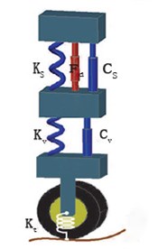
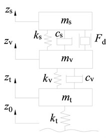
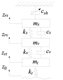
Considering the quarter-car model to be with high accuracy in analyzing the suspension dynamics, it is employed to model the semi-active suspension in this paper. Fig. 1 presented a three DOF model of quarter-car suspension system containing the seat suspension with a MR damper. In this figure the car body, seat and human body are included as the sprung masses: and , and the vertical dynamics of tire and axle is often considered by introducing an unsprung mass and spring . MR damper is placed between the seat and the car body to form the seat suspension together with a spring and a damper.
Based on Newton second law, the dynamic equations of seat suspension system is:
where , and are unsprung mass, quarter car body mass and seat (plus human body) mass respectively. , and are the stiffness coefficients of the tire, quarter car suspension and seat suspension respectively. and are the damping coefficients of quarter car suspension and seat suspension respectively. is the semi-active damping force created by the MR damper. , , and are the road excitation, vertical displacements of car axle, body and seat, respectively.
Based on Eq. (1), the state equation of the system is:
where:
Fig. 1Model of quarter-car suspension
2.2. MR damper modeling and analysis
Bouc-wen hysteresis model paralleled with dashpot and spring is originally used to formulate the MR damper. It can describe the hysteretic nonlinearity of the MR damper, but it is unable to describe the nonlinear and saturation dependence of the magnetic field yielded by the direct drive current. A modified Bouc-wen hysteresis model, proposed by Spencer [32], effectively overcomes the above drawback and precisely describes the nonlinear saturated characteristic of the MR damper. The modified Bouc-wen hysteresis model is presented in Fig. 2 and it is finally obtained by adding a serial viscous damping with the Bouc-wen model and further paralleling a linear spring to the serialized structure.
Fig. 2Modified Bouc-Wen model of MR damper
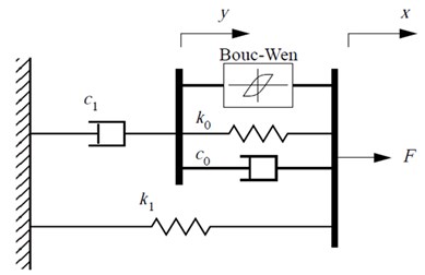
In this paper, the modified Bouc-Wen model is used to describe the mechanical properties of the MR damper. The model introduces two internal variables, and it constructs a differential equation model with 14 parameters to be determined. According to Fig. 2, the mathematical equations of the modified Bouc-wen model are presented as follows:
where , is the stiffness of the damper accumulator. is the viscous damping observed when larger velocities is represented. is a dashpot, included in the model to produce the roll-off that was observed in the experimental data at low velocities. is presented to control the stiffness at large velocities, and is the initial displacement of spring is associated with the nominal damper force due to the accumulator. is given as the output of a first-order filter. is the commanded voltage sent to the current driver.
As for the RD-1005-3 damper produced by Lord Corporation, its parameters are chosen as follows. 963 N/cm, 53N·S/cm, 14 N/cm, 930 N·s/cm, 5.4 N/cm, 200 cm2, 200 cm-2, 2, 207, and 18.9 cm, the response of the proposed model at 2.5 Hz is obtained as shown in Fig. 3. It can be seen from Fig. 3 that MR damper can provide the damping effect in the plane of I and III quadrant of velocity-force plane, unlike the active actuator in all the four quadrants. Therefore, the output of MR damper has to track the desired damping force only when the expected force and velocity have same sign, otherwise it should output the least damping force, so the formula described is:
where is the damping force of MR damper, is the desired force which is obtained by using suspension controller, is the minimal damping force corresponding to the zero input current, however it is not a constant value changing with the instant velocity.
If the MR damper controller employs the switching control method of Eq. (6), the input voltage of the MR damper switches between the minimum and maximum without being a continuous adjustable control signal, which limits the performance of the MR damper. In this paper neural network is used to simulate the inverse model of MR damper, and it is further be as the nonlinear controller of MR damper to create a continuous signal for MR damper, which will be discussed in next section.
Fig. 3Experimentally obtained response of the model
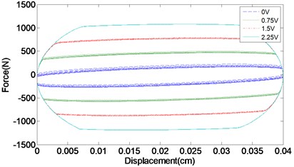
a) Force vs. displacement
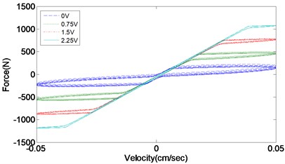
b) Force vs. velocity
2.3. Neuro inverse model approximating of MR damper
The reverse model of MR damper is defined as solving the voltage corresponding to input MR damper after the desired damping force is obtained by FSMCEF control algorithm. The aim of the reverse model is to make MR damper track this desired force as possible. The inverse model can be described using the following nonlinear function:
where is the input voltage, namely the output of MR damper reverse model. is the neural network weight vector, determined by training process. is the input vector as , in which is the th(current) time step, , and are the previous time step numbers of input voltage, damping force and displacement respectively.
The BP neural network can approximate an arbitrary nonlinear continuous function with arbitrary precision, and it is used for the inverse-dynamics approximation of MR damper is shown in Fig. 4.
Fig. 4Block diagram of neuro inverse dynamics model for MR damper
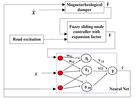
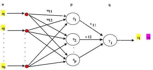
The typical BP network is divided into three layers, which are input layer, hidden layer and output layer. For the inverse dynamics model of Eq. (7), the network input layer is set with 9 nodes and the hidden layer with 20 nodes (see Fig. 5, 20), the output layer has one node, standing for the input voltage of the MR damper.
The output of the hidden node is:
The output of the output node is:
Fig. 5Detailed neural network for the inverse dynamics approximation
This neural network training includes namely mode suitable transmission, error back propagation, memory training and learning convergence. The detailed training procedures are as follows.
(1) Initialization:
The weights of , and threshold of , are all set as random values in (–1, 1).
(2) Randomly pick up a pair of samples for network training.
(3) Calculate the output of the hidden layer using Eq. (8).
(4) Calculate the output layer using Eq. (9).
(5) Calculate the average error of the output layer: .
(6) Calculate the hidden layer general error: .
(7) Modify the output layer weights and thresholds:
(8) Modify hidden layer weights and thresholds:
(9) Take out the next pair of sample and return Step (3) to repeat until completing all training samples.
(10) Determine whether a global error is less than the preset value, otherwise, to return to Step (2) to continue until meeting the requirements.
The displacement and the input voltage, as the network input, are generated by Gaussian white noise with frequency ranges of 0-3 Hz and 0-4 Hz respectively. A data set of 10000 points used for training and validation are created by 500 Hz sampling frequency in 20 s sample time. These data are used for training the network and another data set including 1200 points is further created to validate the training. The BP neural network training and validating process is shown in Fig. 6 and the control voltage between the predict output and desired output shown in Fig. 7. The BP network prediction error compared with the desired output is shown in Fig. 8.
Fig. 6BP neural network training and validating process
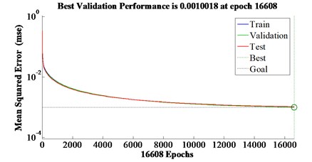
Fig. 7Control voltage between the predict output and the desired output
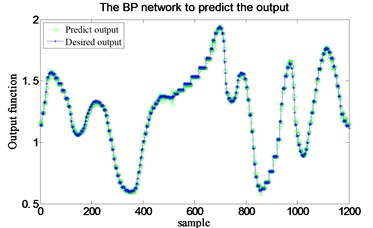
Fig. 8BP network prediction error
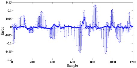
Table 1BP predict output data, desired output data and their errors
Sample No. | Predict output | Desired output | Errors |
1 | 1.154196198 | 1.139969109 | 0.014227089 |
2 | 1.144247759 | 1.139969109 | 0.00427865 |
3 | 1.141656099 | 1.139969109 | 0.00168699 |
4 | 1.140767273 | 1.139969109 | 0.000798164 |
5 | 1.140462485 | 1.139969109 | 0.000493376 |
6 | 1.140385454 | 1.139969109 | 0.000416345 |
7 | 1.140396186 | 1.139969109 | 0.000427077 |
8 | 1.151196722 | 1.235470511 | –0.084273789 |
9 | 1.219608674 | 1.235470511 | –0.015861836 |
10 | 1.242757353 | 1.235470511 | 0.007286842 |
11 | 1.228802917 | 1.235470511 | –0.006667594 |
12 | 1.228274434 | 1.235470511 | –0.007196077 |
13 | 1.229949686 | 1.235470511 | –0.005520825 |
14 | 1.231869009 | 1.235470511 | –0.003601502 |
15 | 1.227968248 | 1.326840347 | –0.098872098 |
…… | …… | …… | …… |
1.140153642 | 1.135359005 | 0.004794637 | |
1195 | 1.140148274 | 1.135359005 | 0.00478927 |
1196 | 1.140113462 | 1.135359005 | 0.004754457 |
1197 | 1.140047649 | 1.135359005 | 0.004688644 |
1198 | 1.139997841 | 1.135359005 | 0.004638836 |
1199 | 1.139988131 | 1.135359005 | 0.004629127 |
1200 | 1.108848138 | 1.115573823 | -0.006725686 |
Table 1 shows the BP predict output data, the desired output data and their error. The sum of the absolute value of 1200 errors is 15.9525. Table 1 presented the detailed result of some samples, and the results show that the BP neural network predict output values substantially agree with the actual situation, and the errors are small, demonstrating that this model is highly with the project reality and the neural network model is effective.
3. Fuzzy sliding mode controller design
The difference of sliding mode variable structure control from other conventional control strategies is its discontinuity of control. the system structure make switch characteristics change over time, and that control features can force the system make small amplitude and high frequency movement up and down along the switching surface, which called “sliding mode” (see Fig. 9). The sliding mode can be designed irrelative with parameter perturbation and external disturbance, and the system under sliding mode has good robustness.
Fig. 9Sliding mode motion in 2-D phase plot
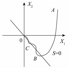
But the sliding mode motion under parameters perturbation and external disturbance is easy to cause the high frequency chattering, because the high frequency chattering is infinitely fast in theory, but in practice no actual actuators can realize it. The chattering phenomenon gives rise to the application difficulties of sliding mode control. In the next sections, the sliding mode controller for semi-active suspension will be designed and its combination with fuzzy logic will further completed to depress the chattering. The sliding mode controller takes an ideal skyhook model as the reference, and creates a sliding mode control law based on the errors dynamics between the seat suspension and its reference model. Thus, the skyhook model is first established and the next is discussing the errors dynamics. Further fuzzy rules are used to suppress the chattering occurred in the above sliding mode control by fuzzifying the sliding mode surface and its derivative. Considering that the chattering results in the errors changing in a large range, an expansion factor is used to change the universe of the fuzzy logic but without changing the fuzzy rules, which forms a new variable universe fuzzy controller with adaptive characteristic. The combining of the sliding mode controller and fuzzy controller with expansion factor is further studied, the new formed FSMCEF design is presented and its stability further completed.
3.1. Skyhook reference model
Herein the skyhook model is used as the reference to form the fuzzy sliding control algorithm, and it is presented in Fig. 10.
The dynamics equations are derived based on Newton second law as follows:
where , and are the road excitation, vertical displacements of unsprung mass, car body and seat respectively, which are the corresponding variables in the reference system compared with the plant system in Fig. 1. is the damping coefficient of “sky-hook” damper.
Fig. 10Skyhook reference model
The state vector for the reference system is taken as , and the output vector is taken as . According to Eq. (12) the state equations are established as:
where:
3.2. Error dynamics model used for SMC and FSMCEF
Both the sliding mode controller and the fuzzy sliding mode controller are designed to make the actual seat suspension motion to track the reference mode, and so they are based on the dynamic errors between the seat suspension and the skyhook reference model. Based on the above seat model and the reference model, the seat suspension displacement error, its integral and its differential (velocity error) are taken as the control variables, and they form the general tracking error vectoras and its differential is . so, the error dynamic equation is obtained as:
where:
3.3. Sliding mode control based on pole placement
The switching surface is taken as:
As for , Eq. (14) can be written to partitioned matrix form as:
As for , Eq. (16) can be written as:
The characteristic polynomial for Eq. (18) is . To obtain the value of and , its characteristic roots are equal to the given poles.
The chief problem of pole assignment is rationally to determine the desired closed-loop poles set. The standard form of the second-order system transfer function is:
The two closed-loop poles are , and the system works in less damping state () which makes these two poles to be conjugate complex roots located in the left half plane of domain and to have the appropriate oscillation and short transition process. For the three orders system are in Eqs. (16) and (17), the desired poles number are 3. The conjugate pole pair of and are selected as the dominant poles, and the third is a non-dominant one. The poles placement of our closed-loop system is completed to ensure the two dynamic performance indices: peak time and overshoot %. These two indices are set as 15 %, 0.7, which determines the dominant poles be at –2.7326±4.4886i and the non-dominant pole at –20. The corresponding parameters are and . So, the switching function coefficient vector is . The system performance is mainly determined by these two dominant poles and the non-dominant pole only produces minimal effect.
When system is in sliding mode motion, , and:
The equivalent control for system into fuzzy sliding mode or sliding mode is , and:
In order to improve the dynamic quality of the movement, the approaching mode employs the constant speed reaching law as:
where 3.
The final sliding mode control law is taken as:
So, the desired real-time variable damping force is as:
where , 3.
3.4. Fuzzy sliding mode control
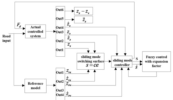
The fuzzy logic control is further added to overcome sliding mode controller “chattering” problem. The connection of the sliding mode controller and the fuzzy logic controller is shown in Fig. 11, which formed the final fuzzy sliding mode controller. The detailed content of the fuzzy control block in Fig. 11 is presented in Fig. 12. Its inputs are and , with one output sent to the sliding mode controller.
Fig. 11Block diagram of FSMCEF system
The fuzzy controller first change the range of and , namely from their original ranges of [–0.04, 0.03] and [–6×10⁻³, +8×10⁻³] both to the new range of [–6, +6] for further discretization and fuzzification. The corresponding conversion equation is:
Fig. 12The structure of fuzzy controller
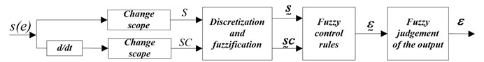
The variables after conversion are and (Fig. 12), and they are further discretized and fuzzified to form fuzzy sets , . In this process and are classified into seven grades, forming seven fuzzy subsets, including: NL (Negative Large), PL (Positive Large), NM (Negative Medium), PM (Positive Medium), NS (Negative Small), PS (Positive Small), NE (0). The and of domain and are belonging to 7 fuzzy subsets, respectively. Similarly, the output value are also ranked into seven fuzzy subsets: NL, PL, NM, PM, NS, PS, NE.
For this double input and single output fuzzy controller, the control rules can be written as the following form: If and then , (1, 2,…, 7, 1, 2,.., 7), where , are input fuzzy sets, and is output fuzzy sets.
These fuzzy sets conditional statements can be summed up in a fuzzy relation , and . According to each inference rules, the corresponding fuzzy relations, can be calculated. So, the total of the whole system corresponding fuzzy control rule is:
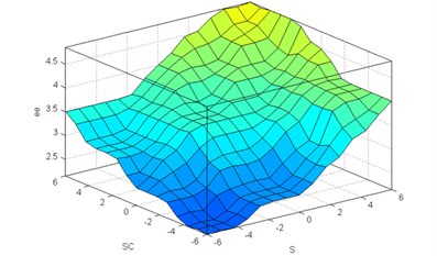
The final fuzzy rules are shown in Table 2, and according to Table 2 the 3-D input-output relation diagram of the fuzzy controller is obtained as shown in Fig. 13.
Table 2Fuzzy rules
NL | NM | NS | ZE | PS | PM | PL | ||
NL | NL | NL | NM | NM | NS | NS | ZE | |
NM | NL | NL | NM | NS | NS | NS | ZE | |
NS | NM | NM | NS | ZE | ZE | ZE | ZE | |
ZO | NM | NM | NS | ZE | ZE | PS | PS | |
PS | NS | NS | ZE | ZE | PS | PS | PM | |
PM | ZE | PS | PS | PS | PS | PM | PL | |
PL | PS | PS | PS | PM | PL | PL | PL | |
Fig. 133-D diagram of Fuzzy control rules
When is determined, according to , and synthetic fuzzy reasoning rules, the corresponding fuzzy sets of controls is , and:
The final fuzzy sliding or sliding mode control law is taken as:
3.5. Fuzzy sliding mode control with expansion factor
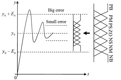
Equidistant domain partitioning method is used in fuzzy control generally. When the error is large, the system has sufficient error resolution, and it is shown as the “big error” dotted line in Fig. 14. When the error is small, the system response only changes around “ZO” corresponding to the original fuzzy partition, and other fuzzy subsets obviously do not work. Ideally, when the error is reduced, the domain of the fuzzy controller should be able to make self-adaptation adjustment. The accuracy of the fuzzy controller is related to the number of output variables and fuzzy rules. Supposing the input is -dimensional, the fuzzy control rule of the universe is divided into ; the total rule number is , if the fuzzy subset of the domain is divided into smaller, the number of fuzzy control rules will increase exponentially, increasing the difficulty of making rules. Therefore, under the premise of not affecting the control effect, we should try to use less fuzzy subset to reduce the number of fuzzy control rules. With the same form of rules, the universe shrinks as the error becomes smaller, and the universe expands as the error increases. The contraction of the domain is equivalent to increasing the fuzzy control rules to improve the control accuracy. The function of the scaling factor transforms the domain into , where is a continuous function of the error variable . The appropriate domain expansion factor is chosen so that the range of the universe changes with the error, which can realize the adaptive implementation of the expansion of the domain, without the need for other auxiliary algorithms and increase the control rules.
Fig. 14Adjustment of the domain
Let be the universe of input variable , is the universe of output variable ; is the fuzzy partition on , is the fuzzy partition on , . As , are the linguistic variables, fuzzy inference rule can be formed:
where is peak, and is peak , , The fuzzy control system of Eq. (31) can be expressed as an -piece piecewise interpolation function:
The variable universe is that domain and can be adjusted independently with the change of input variable and output , respectively:
where and is the domain expansion factor. In contrast to the variable universe, the original universe and is called the initial universe. Eq. (32) can be expressed as -piece dynamic interpolation function:
where , and is chosen as:
or:
In this paper , 104. is chosen as:
where is the proportionality constant, and is according to the actual situation, usually try 1. The control law of the variable universe fuzzy controller is:
, is two-dimensional input domain, respectively, and is the output domain. When and are relatively independent, we can get the expansion factor , and expansion factor . But in most cases, and are related. If is the error domain and is often the domain of error variation, and should be defined on and , then the input and output of the domain expansion factor are:
Since the error variation depends on the error, can be simply taken as , Eq. (41) can be rewritten as:
3.6. Stability analysis
3.6.1. Stability analysis of nominal system based on Lyapunov theorem
The poles placement of our closed-loop system is completed to ensure the two dynamic performance indices: peak time and overshoot %. These two indices are set as %, which determine the dominant poles be at –2.7326±4.4886i and the non-dominant pole at –20. The corresponding parameters are and . So, the switching function coefficient vector is . The energy function is taken as and it is positive definite, and its differential , namely negative definite, so the entire system is asymptotically stable.
3.6.2. Robust stability analysis of system under parameter uncertainty and external disturbance
Considering the general form of the linear uncertainty system is:
where are uncertainty matrix of A and B respectively, which describes the differences between the nominal value of parameters and the actual true values; is the uncertainty of disturbance. Without loss of generality, the nominal model of the controlled object Eq. (43) is supposed to be completely controllable.
In order to study the impact of various uncertainties on the control system, , and can be decomposed into:
where , ; , , , .
The first term on the right-hand side of Eq. (44) satisfies the matching condition and is the matching part of the uncertainty factor; the second term is the residual part, which is the mismatching uncertainty factor. Generally, the information easy to obtain for the uncertainty factor is its lower and upper bounds.
Hypothesis 1: The uncertain factors of the controlled object Eq. (43) are bounded:
where , , are known constants.
When , and are equal to zero respectively, Eq. (44) is equivalent to uncertainty factor matching conditions or invariance conditions:
The controlled object Eq. (43) is the matching uncertainty system; when either , or is established, the controlled object is a linear mismatch uncertainty system.
For the linear mismatch uncertainty system described by Eq. (43), the design of m-dimensional sliding mode domain in n-dimensional state space is as:
In order to guarantee the non-singularity of the variable structure control system, the sliding mode requirement is . Thus, by the equivalent control method, the state equation of the variable structure closed-loop equivalent system of the mismatched uncertain Eq. (43) can be deduced:
Due to when is bounded, mismatch perturbation uncertainty factor has nothing to do with stability, so lose the generality: . And mismatch parameters and input uncertainty factors are introduced the equivalent system and will cause the disturbance of its Eigen values, affecting the dynamic characteristics and stability of closed-loop system. The stability and robustness of the variable-structure closed-loop control system Eq. (49) will be studied by estimating the perturbations of and to the eigenvalues.
1. When (, 0).
For a variable structure equivalent system Eq. (48):
When , ; has nonzero single eigenvalues , ,…, .
(1) There is always a similarity transformation matrix , and:
(2) Because the eigenvalue has invariance to matrix similarity transformation, all the disturbance of the characteristic value caused by to is transformed into the disturbance of to in Eq. (50). Let , and . Then by Gerschgorin in the theorem, for each there is always :
and:
and:
The above equation shows that the existence of parameter mismatch uncertainty factor makes the eigenvalue of the equivalent system change from , ,…, to , ,…, , and all the values of the eigenvalue (single or multiple) are in the union of circles with as the radius.
The sufficient condition for the asymptotic stability of the variable structure equivalent systems is given by Eq. (49). To substitute Eq. (53) into the equation, the sufficient condition becomes .
A sufficient condition for the asymptotic stability of the variable structure equivalent system Eq. (49) is given as:
where , is absolute.
2. When (, ).
is as a mismatching input uncertainty factor, and the effect of disturbance on the eigenvalue and stability of the variable structure equivalent system is more complicated than that of the mismatch parameter uncertain factor , and with the control of the variable structure control system law intertwined. According to the characteristics of nonlinear discontinuous feedback in variable structure control systems, the control law has the general form:
where , and are the quiver factors.
For a variable structure equivalent system:
Given that , and have single nonzero eigenvalues, then the sufficient conditions for the asymptotic stability of the equivalence system is:
where .
3. When and (, ).
For linear mismatched uncertain system Eq. (43), the sliding mode is Eq. (47), and the variable structure control law is given by Eq. (55), if has nonzero single eigenvalues , ,…, ; then the sufficient conditions for large-scale asymptotic stability of variable structure equivalent systems is:
where and are definitude respectively.
4. Numerical simulation and performance analysis
To evaluate the effectiveness of the proposed FSMCEF, A Simulink model is completed according to a certain model of car parameters which are shown in Table 3. For comparison, the FSMCEF, SMC, PID and passive mode are established for the same model.
The road input is where is the vertical displacement for pavement input; is the cut off frequency for road input; is the road roughness coefficient; is the speed; is the input white noise. Simulation parameter settings are as follows: 6.4×10⁻³ m3, 20 m/s, 0.01 Hz. Fig. 15 presented the FSMCEF simulink model without MR of quarter-car seat suspension system. Fig. 16 is the result of comparing the proposed FSMCEF with the sky-hook reference model. It displays that the FSMCEF can effective track the sky-hook reference mode.
Table 3parameters of a certain model of car
Parameter | Value | Unit |
80 | kg | |
400 | kg | |
40 | kg | |
8000 | N/m | |
250 | N/(m·s-1) | |
700 | N/(m·s-1) | |
2000 | N/(m·s-1) | |
18500 | N/m | |
1500 | N/(m·s-1) | |
185000 | N/m | |
2-5 | – |
Fig. 15FSMCEF Simulink model with MR of quarter-car seat suspension system
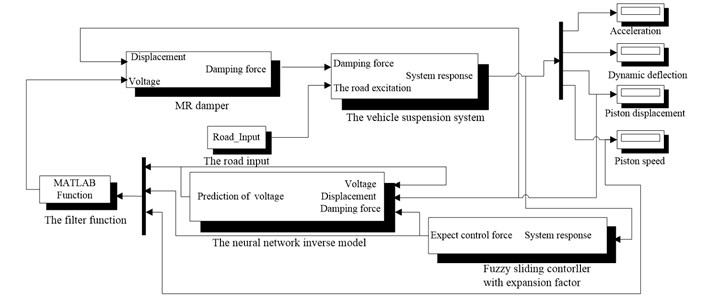
Fig. 16Comparing the proposed FSMCEF with the sky-hook reference model
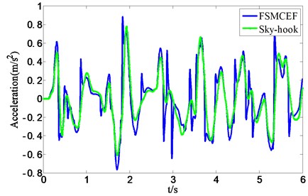
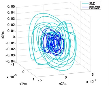
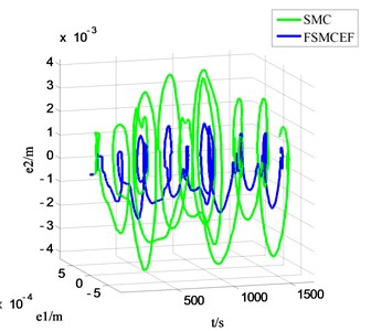
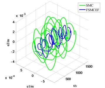
Fig. 17, Fig. 18 and Fig. 19 are the --, -- and -- phase diagram of fuzzy sliding with expansion factor and sliding mode movement respectively, and every figure has two different view angle parameters: azimuth (AZ) and elevation (EL). In the beginning with , and are in the system initial states, and the defaults are zeros, through the results can be seen in the graph, each cycle system is able to achieve balance, and it can be seen that FSMCEF can effectively restrain the chattering.
Fig. 17The e1-e2-e3 phase diagram of FSMCEF and SMC
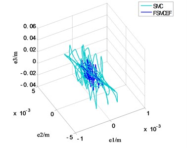
a) AZ: –29 EL:42
b) AZ:70EL:16
Fig. 18The t-e1-e2 phase diagram of FSMCEF and SMC
a) AZ: –18 EL:10
b) AZ: –49 EL:34
Fig. 19The t-e2-e3 phase diagram of FSMCEF and SMC
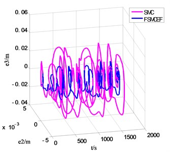
a) AZ: –14 EL:20
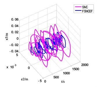
b) AZ: –33 EL:44
In order to verify the effectiveness of MR damper neural network-based inverse dynamics model, the Simulink model of seat suspension without neural network-based inverse dynamics model is further built as shown in Fig. 20, and Fig. 21 and Fig. 22 demonstrated the acceleration and force of FSMCEF controller with and without the inverse dynamic model of MR damper. It can be seen from the experimental results that the neural network model is used to simulate the inverse dynamic characteristics of the MR damper for the highly nonlinear characteristics of the MR damper. The neural network model directly provides the desired control force for the generation of the fuzzy sliding mode with expansion factor to obtain a continuous input voltage, and can be seen that FSMCEF controller with the inverse dynamic model of MR damper can effectively follow the ideal FSMCEF controller.
To testify the performance of FSMCEF, other control methods including SMC, PID and passive suspension (no control) are also simulated as the comparisons. Fig. 23 and Fig. 24 presented the simulation results of all the above methods. It can be seen that FSMCEF is much better than SMC, PID and passive mode at both acceleration and deflection aspects.
Fig. 20FSMCEF Simulink model without MR of quarter-car seat suspension system
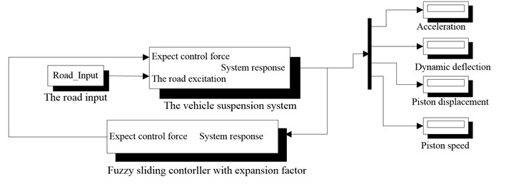
Fig. 21Force result of FSMCEF with and without the inverse dynamic model of MR damper
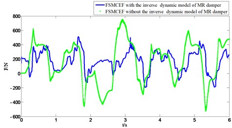
Fig. 22Acceleration result of FSMCEF with and without the inverse dynamic model of MR damper
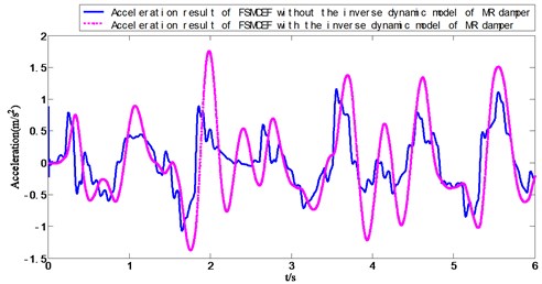
Table 4 and 5 presented the standard deviation (STD), maximum (max), minimum (min), mean value (mean) and Root Mean Square (RMS) of the deflection and acceleration of seat suspension under different controllers. It can be seen that using FSMCEF the STD, max, min, mean and RMS of seat deflection and acceleration are all the best, compared with using SMC, PID and passive mode. The simulation results are analyzed statistically, Table 6 and Table 7 presented the performance improvement of FSMCEF compared with other methods when employed in seat suspension. It can be seen that FSMCEF is the best controller, and improves the riding comfort and ride comfort.
Fig. 23Simulation result of seat dynamic deflection
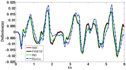
Fig. 24Simulation results of seat acceleration
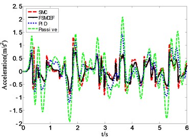
Table 4Statistics results of seat deflection
Controller type | mean / m | STD / m | max / m | min / m | RMS / m |
Passive mode | 0.0084 | 0.0105 | 0.0228 | –0.0243 | 0.0104 |
PID | 0.0079 | 0.0098 | 0.0223 | –0.0226 | 0.0097 |
SMC | 0.0069 | 0.0085 | 0.0183 | –0.0208 | 0.0084 |
FSMCEF | 0.0068 | 0.0083 | 0.0182 | –0.0202 | 0.0082 |
Table 5Statistics results of seat acceleration
Controller type | mean / m·s-2 | STD / m·s-2 | max / m·s-2 | min / m·s-2 | RMS / m·s-2 |
Passive mode | 0.4746 | 0.6283 | 2.3419 | –1.8309 | 0.6281 |
PID | 0.4186 | 0.5574 | 1.9041 | –1.5512 | 0.5573 |
SMC | 0.3416 | 0.4179 | 1.3151 | –0.9721 | 0.4179 |
FSMCEF | 0.2506 | 0.3040 | 0.8860 | –0.7641 | 0.3042 |
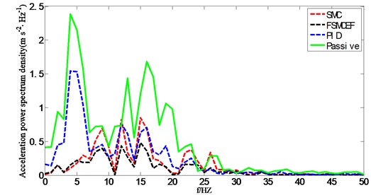
From Table 6 it can be concluded that FSMCEF outperforms the other their control methods, especially with 51.57 % improvement relative to the traditional seat suspension in passive mode. Further, the frequency domain performance of FSMCEF is verified, and the seat suspension acceleration power spectrum density under the random road excitation is shown in Fig. 25. It is shown that FSMCEF improves significantly the ride comfort of vehicle in lower frequency compared with the SMC, PID and passive seat acceleration, and it improves the vehicle ride comfort. In vehicle body resonant vibration range (1-1.5 Hz) and the low-mid frequency range (4-12.5 Hz) which human body is sensitive to, the FSMCEF also can effectively reduce the seat acceleration. So, the FSMCEF effectively reduces the vehicle vibration influence on the human body, significantly improves the dynamic comfort of vehicle systems.
Table 6The performance deflection improvement of FSMCEF compared with other methods
Controller type | mean | STD | RMS |
FSMCEF vs Passive mode | 19.05 % | 20.95 % | 21.15 % |
FSMCEF vs PID | 13.924 % | 15.31 % | 15.46 % |
FSMCEF vs SMC | 1.45 % | 2.35 % | 2.38 % |
Table 7The performance acceleration improvement of FSMCEF compared with other methods
Controller type | mean | STD | RMS |
FSMCEF vs Passive mode | 47.19 % | 51.62 % | 51.57 % |
FSMCEF vs PID | 40.13 % | 45.46 % | 45.42 % |
FSMCEF vs SMC | 26.63 % | 27.26 % | 27.21 % |
Fig. 25Acceleration power spectrum density of seat suspension under random road excitation
5. Conclusions
In this paper, a fuzzy sliding mode controller with expansion factor (FSMCEF) is designed for the MR damper-based semi-active seat suspension. This FSMCEF takes the sky-hook model as the reference, and can guarantee the output of MR damper to be effective damping when the motion direction frequently changes. Aiming at the high nonlinearity of MR damper, the neural network model is used to simulate the inverse dynamic characteristic of MR damper. The neural network model directly provides the expected control force to generate the fuzzy control sliding-mode expansion factor to obtain continuous input voltage. The FSMCEF is derived based on the error dynamics of the skyhook and the controlled plant, and its fuzzy control term can attenuate the chattering. Considering the hysteresis nonlinearity of MR damper, a three-layer BP neural network is trained to approximate the MR damper’s reverse dynamics and taken as the controller of the MR damper. Numerical simulations verified the effectiveness of the FSMCEF compared with PID control, SMC and passive mode for seat suspensions with same model parameters, and the performance of the vehicle suspension system can be effectively improved by the introduction of the MR damper in the control strategy, and the active control of the MR damper can be realized at the same time.
References
-
Margolis D. L. Procedure for comparing passive active and semi-active approaches to vibration isolation. Journal of the Franklin Institute, Vol. 315, Issue 4, 1983, p. 225-238.
-
Yao G. Z., Yap F. F., Chen G., et al. MR damper and its application for semi-active control of vehicle suspension system. Mechatronics, Vol. 12, Issue 7, 2002, p. 963-973.
-
Nguyen S. D., Nguyen Q. H., Choi S. B. A hybrid clustering based fuzzy structure for vibration control –Part 2: An application to semi-active vehicle seat-suspension. Mechanical Systems and Signal Processing, Vols. 56-57, 2015, p. 288-301.
-
Unger A., Schimmack F., Lohmann B., Schwarz R. Application of LQ-based semi-active suspension control in a vehicle. Control Engineering Practice, Vol. 21, Issue 12, 2012, p. 1841-1850.
-
Hac A., Youn I. Optimal semi-active suspension with preview based on a quarter car model. Transactions of ASME Journal of Vibration and Acoustics, Vol. 114, 1992, p. 84-92.
-
Nguyen M. Q., Sename O., Dugard L. An LPV fault tolerant control for semi-active suspension – scheduled by fault estimation. IFAC-Papers Online, Vol. 48, Issue 21, 2015, p. 42-47.
-
Martinez T. J. C., Alcantara H. D., Menendez M. R. Semi-active suspension control with LPV mass adaptation. IFAC-Papers Online, Vol. 48, Issue 26, 2015, p. 67-72.
-
SChoi B., Lee H. S., Park Y. P. H∞ control performance of a full-vehicle suspension featuring magnetorheological dampers. Vehicle System Dynamics, Vol. 38, Issue 2002, 5, p. 341-360.
-
Guo D. L., Hu H. Y., Yi J. Q. Neutral network control for semi-active vehicle suspension with a magneto-rheological damper. Journal of Vibration and Control, Vol. 10, Issue 3, 2004, p. 461-471.
-
Yao G. Z., Yap F. F., Chen G., et al. MR damper and its application for semi-active control of vehicle suspension system. Mechatronics, Vol. 12, 2002, p. 963-973.
-
Dyke S. J., Spencer B. F. A comparison of semi-active control strategies for the MR damper. Intelligent Information Systems, Vol. 8, Issue 10, 1997, p. 580-584.
-
Dyke S. J., Spencer B. F., Sain M. K. Modeling and control of magneto-rheological dampers for seismic response reduction. Journal of Smart Materials and Structures, Vol. 5, 1996, p. 565-575.
-
Bin Gu, Sheng Victor S. A robust regularization path algorithm for ν-support vector classification. IEEE Transactions on Neural Networks and Learning Systems, 2016, https://doi.org/10.1109/TNNLS.2016.2527796.
-
D’Amato F. J., Viassolo D. E. Fuzzy control for active suspensions. Mechatronics, Vol. 10, Issue 8, 2000, p. 897-920.
-
Miao Y., Qu W., Qiu Y., Zhang L. An adaptive fuzzy controller for vehicle active suspension systems. Automotive Engineering, Vol. 23, Issue 1, 2001, p. 9-12.
-
Kim C., Ro P. I. A sliding mode controller for vehicle active suspension systems with non-linearities. Proceedings of the Institution of Mechanical Engineers, Part D: Journal of Automotive Engineering, Vol. 212, Issue 2, 1998, p. 79-92.
-
Sam Y. M., Osman J. H. S., Ghani M. R. K. A class of proportional-integral sliding mode control with application to active suspension system. Systems and Control Letters, Vol. 51, Issues 3-4, 2004, p. 217-23.
-
Yagiz N., Yuksek I. Sliding mode control of active suspensions for a full vehicle model. International Journal of Vehicle Design, Vol. 26, Issues 2-3, 2001, p. 264-76.
-
Zheng Yuhui, Jeon Byeungwoo, Xu Danhua, Wu Q.M. Jonathan, Zhang Hui Image segmentation by generalized hierarchical fuzzy C-means algorithm. Journal of Intelligent and Fuzzy Systems, Vol. 28, Issue 2, 2015, p. 961-973.
-
Wen Xuezhi, Shao Ling, Xue Yu, Fang Wei A rapid learning algorithm for vehicle classification. Information Sciences, Vol. 295, Issue 1, 2015, p. 395-406.
-
Yoshimura T., Kume A., Kurimoto M., et al. Construction of an active suspension system of a quarter car model using the concept of sliding mode control. Journal of Sound and Vibration, Vol. 239, Issue 2, 2001, p. 187-99.
-
Yao J. L., Zheng J. Q., Gao W. J., et al. Sliding mode control of vehicle semi-active suspension with magneto-rheological dampers having polynomial model. Journal of System Simulation, Vol. 21, Issue 8, 2009, p. 2400-2404.
-
Chen Y., Zhao Q. Sliding mode variable structure control for semi-active seat suspension in vehicles. Journal of Harbin Engineering University, Vol. 33, Issue 6, 2012, p. 775-781.
-
Spencer R. B. F., Dyke D. J., Sain K. M., et al. Phenomenological model of a magnetorheological damper. Journal of Engineering Mechanics, Vol. 123, Issue 3, 1997, p. 230-238.
-
Berstecher R. G., Palm R., Unbehauen H. D. An adaptive fuzzy sliding mode controller. IEEE Transactions on Industrial Electronics, Vol. 48, Issue 1, 2001, p. 18-31.
-
Chen C. S., Chen W. L. Robust adaptive sliding mode control using fuzzy modeling for an inverted pendulum system. IEEE Transactions on Industrial Electronics, Vol. 45, Issue 2, 1998, p. 297-306.
-
Ha Q. P., Nguyen Q. H., Rye D. C., Durrant-Whyte H. F. Fuzzy sliding-mode controllers with applications. IEEE Transactions on Industrial Electronics, Vol. 48, Issue 1, 2001, p. 38-46.
-
Lee H., Kim E., Kang H. J., Park M. Design of a sliding mode controller with fuzzy sliding surfaces. IEE Proceedings – Control Theory and Applications, Vol. 145, Issue 5, 1998, p. 411-8.
-
Lin F. J., Chiu S. L. Adaptive fuzzy sliding mode control for PM synchronous servo motor drives. IEE Proceedings – Control Theory and Applications, Vol. 145, Issue 1, 1998, p. 63-72.
-
Lin Jeen, Lian Ruey-Jing, Huang Chung-Neng, Sie Wun-Tong Enhanced fuzzy sliding mode controller for active suspension systems. Mechatronics, Vol. 19, 2009, p. 1178-1190.
-
Li H.-X. The mathematical essence of fuzzy controls and fine fuzzy controllers. Advance in Machine Intelligence and Soft-Computing, Vol. 4, 1997, p. 55-74.
-
Spencer R. B. F., Dyke D. J., Sain K. M., et al. Phenomenological model of a magnetorheological damper. Journal of Engineering Mechanics, Vol. 123, Issue 3, 1997, p. 230-238.
Cited by
About this article

The research work is supported by Heilongjiang Province Science Foundation (Grant No. LC2015019) and supported by the Fundamental Research Funds for the Central Universities (Grant No. 2572015AB18).
