Shaking table testing and numerical modeling of continuous welded ballast track on bridges under longitudinal seismic loading

2.1. Test purpose

According to existing research (based on the longitudinal track-bridge interaction), the rail longitudinal force under seismic loading is several times larger than that of the temperature condition [13, 15]. Therefore, the seismic effect on rail longitudinal forces should be considered when designing CWR on bridges across the seismic zone. Compared with vertical and transverse seismic vibrations, the longitudinal seismic vibrations have the most direct and important effect on rail longitudinal force. In addition, the track longitudinal resistance is also an important parameter in the structural design of CWR on the bridge. For ballast track, the nonlinearity of track longitudinal resistance under seismic loading is significant, especially under longitudinal seismic loading. Therefore, this paper focuses on longitudinal seismic vibrations, and a test model of continuous welded ballast track on bridges was designed and established, and the following three aspects were investigated.

1) An analysis of the influence of bridge motion caused by earthquakes on the performance of granular ballast beds and its resistance;

2) A study of the changing longitudinal rail forces under seismic loading;

3) A verification of the rationality of the ideal elasto-plastic resistance model applied to the ballast track under seismic loading, which can be used as a reference for modifying the theoretical model.

2.2. Seismic response simulator

A test was carried out with a strong earthquake response simulator machine. The specifications of which are as follows:

Table size: 7.0 m×2.0 m (a design especially extended for this test); shaking direction: horizontal single direction; Max. Stroke: ±100 mm; Max. Acc: 1.2 g; Weight limit: 25 ton.

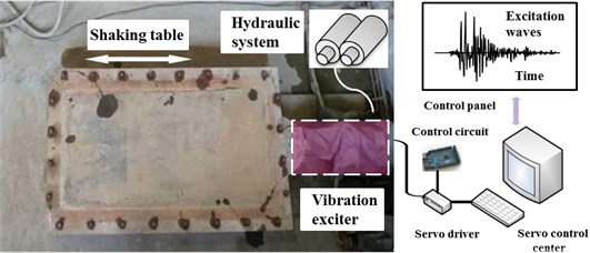
The experimental earthquake response simulating test consists of servo control system, shaking table, support system, vibration exciter system, and hydraulic system. In this paper, the experimental test used the acceleration as control signals to control the shaking table. The seismic acceleration waves were input as excitation by the servo control system, and the parametric generator converted the seismic waves into the acceleration parameter signals and control the movement of the shaking table through the servo controller, as shown in Fig. 1.

Fig. 1Strong earthquake response simulator

2.3. Test model

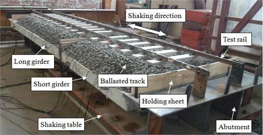
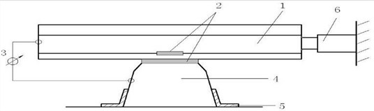
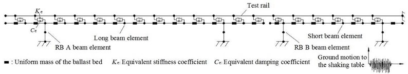
As shown in Fig. 2, the test model consists of the ballast track, two beams of different lengths, and the adjacent abutment part. The bridge beams were RC slab boards of 2.0 m in length×2.0 m in width×0.20 m in height and 3.9 m in length×2.0 m in width×0.20 m in height, which were supported by rubber bearings fixed on the shaking table. The abutment was a rigid steel frame, tightly fastened to the table, and the total weight of the model was about 13 tons.

Fig. 2Test model

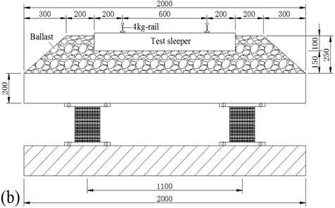
The detailed design of the model is shown in Fig. 3. The scaled rail (4kg rail track), with the sectional area of 5.1 cm² and length of 7 m, was fixed to the abutment at one end and free at the other end. Microcellular rubber pads were placed between the rail and sleeper and strongly held by special fasteners so as to ensure there was no relative displacement between the rail and sleeper. The ballast bed was 1.4 m in top width, 2.0 m in bottom width, and 0.15 m in height, with a size distribution of 10.5-31.5 mm. Furthermore, the ballast bed weighed 655 kg per meter including rail and sleeper, and the bridge beams weighed 4134 kg and 2120 kg respectively. In order to simulate the actual structure of the bridge, the beam was supported by four rubber bearings; the design parameters of the bearing are shown in Table 1. Among them, the long beam was supported by RB A, and the short beam was supported by RB B. In the test model, the ballast resistance at the beam gap was ignored, and a holding sheet was set to prevent the scatter of ballast.

Fig. 3Schematic view of test setup

a) Model front view

b) Model cross section S-S

2.4. Sensor layout

For the shaking table model test, three acceleration sensors, two displacement sensors and twenty rail strain gauges were arranged, the sensor layout illustration is shown in Table 2. The model loading control and data collection system features actuator, sensor, and data collection units [11, 14]. The actuator units are controlled with an electrohydraulic servo driven HS-25t seismic simulation platform, and the sensor units are comprised of a force and displacement sensors. In addition, rail stress is measured with a resistance strain gauge, and a CW-YB-2 displacement sensor (range: ±50 mm, accuracy: 0.01 mm). For the data collection unit, the DHDAS dynamic signal analyzer is used for real-time data collection and recording. The seismic wave input by the actuator of the seismic simulation vibration platform is recorded accurately with a high-precision acceleration probe.

2.5. Loading method

When discussing the seismic response of CWR on bridges, one of the important tasks is the reasonable selection of seismic waves and three methods are widely adopted as follows [16, 19]:

1) The actual recorded seismic wave at the location of bridge. This method is an ideal situation. In general, it is unrealistic to obtain the actual seismic wave record at the location of bridge.

2) The existing recorded seismic waves in the past inland earthquakes. According to the existing research achievements, the typical El-Centro wave, Kobe wave, WenChuan wave, Taft wave and Tianjin wave etc. are selected as inputs of the ground motions for the study of seismic behavior of bridge structures.

3) Synthetic seismic waves. The seismic waves are synthesized based on the statistical characteristic values of seismic wave spectrum, acceleration peak, and duration time etc.

This paper mainly aims to explore the seismic response characteristics of continuous welded ballast track on bridges under earthquakes. Therefore, among the existing recorded seismic waves, the typical El-Centro seismic wave (America, 1940, NS), Kobe (Japan, 1995, NS) seismic wave and WenChuan (China, 2008, EW) seismic wave were selected as inputs of the ground motions for the model. The ground motion acceleration waves are shown in Fig. 4, with primary frequencies of 1.46 Hz, 1.45 Hz and 2.34 Hz, respectively. When discussing the dynamic response of continuous welded ballast track on bridges under seismic loading, the acceleration peak values were set to 0.1 g, 0.2 g and 0.4 g. The test conditions are shown in Table 3.

Fig. 4Ground motion acceleration waves

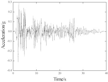
a) El-Centro record

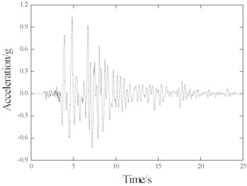
b) Kobe record

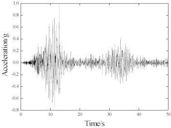
c) Wenchuan record

3.1. Beam longitudinal stiffness

The longitudinal stiffness of the bridge beams was tested after the laying of ballast bed, and the stiffness values were 1.00 kN/mm and 3.85 kN/mm respectively.

3.2. Ballast and fastener longitudinal resistance

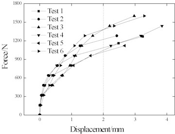
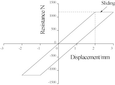
The ballast longitudinal resistance and fastener longitudinal resistance tests are shown in Fig. 5(a) and Fig. 5(b). The ballast average longitudinal resistance was 1186 N with a sliding displacement of 2 mm, as shown in Fig. 6(a). According to assumptions in the existing theory, the ideal elastic-plastic resistance curve is shown in Fig. 6(b). Furthermore, the fastener longitudinal resistance is far greater than the ballast longitudinal resistance, which can be considered as a linear variation, with a linear stiffness of 31 kN/mm.

Fig. 5Test method for ballast and fastener longitudinal resistance

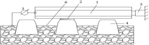
a) Ballast longitudinal resistance test: 1 – test rail; 2 – consolidation component; 3 – displacement meter; 4 – test sleeper; 5 – hydraulic jack; 6 – ballast bed

b) Fastener longitudinal resistance test: 1 – test rail; 2 – special fastener; 3 – displacement meter; 4 – test sleeper; 5 – rigid support; 6 – hydraulic jack

3.3. Beam’s natural frequency and damping ratio

During the shaking table test, one of the most important tasks is to identify the dynamic parameters of the structure, and the sweeping frequency of white noise excitation is the most commonly used method [17]. Before the installation of the test rail, the stationary gauss white noise excitation was input. The bridge beam’s natural vibration frequency was identified by calculating the frequency response function through the measured acceleration record. Additionally, the damping ratio of the first order frequency was calculated by the half-power bandwidth method. The results are shown in Table 4.

The bridge beam natural vibration frequency coincides well with the theoretical results, thereby proving the accuracy of the beam longitudinal stiffness test results. Furthermore, the bridge beam damping ratio coincides well with the natural rubber equivalent damping ratio [18]. In this paper, the damping ratio is taken as 0.03 for calculations.

Fig. 6Ballast longitudinal resistance test results

a) Ballast longitudinal resistance

b) Ideal elastic-plastic resistance

4.1. Numerical model

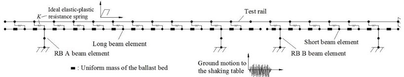
In regards to the continuous welded ballast track on bridges, during testing the ballast bed is subject to a dynamic reciprocating state under seismic loading, a change in the structure between granules will occur, wherein some will flow and redistribute. The dynamic hysteretic change of the ballast longitudinal resistance is complex and quite different from that of the ideal elasto-plastic hysteretic route. Therefore, in order to analyze the influence of nonlinear cyclic hysteretic characteristics of granular ballast beds on the strained state of rail under seismic loading, a CWR on bridge calculation model under seismic excitation is established based on the structural parameters of the test model (see Fig. 7), which can primarily be used to analyze the track-bridge displacement and rail longitudinal stress transmission etc. and perform a contrast analysis with those measured under an ideal elasto-plastic resistance. The longitudinal stiffness and damping ratios of beam supports were measured according to the characteristics of the structural parameters characteristics. In addition, the beam was coupled with the mass of the body itself and the ballast bed (including the ballast, sleeper, and rail), and the total mass of which is a known value. The seismic wave input by the seismic simulation vibration platform was also recorded accurately with a high-precision acceleration probe.

4.2. Vibration equation

When discussing the seismic response of CWR on bridges, due to the strong nonlinearity of structural dynamic responses, the nonlinear time-history step-by-step integration method is adopted [14, 19]. In addition, structural damping is an important dynamic parameter that causes energy dissipation during vibration, thus, the structure’s damping information must be introduced through a reasonable and reliable dynamic finite element analysis model. From a practical point of view, the Orthogonal damping model-Rayleigh method was adopted. The structural vibration equation under seismic loading can be expressed as follows:

Fig. 7Numerical calculation model of test structure

The above equilibrium equation for a nonlinear time interval analysis can be expressed by the following increment within a minor time interval $\mathrm{\Delta }t$:

where $\left[M\right]$, $\left[C\right]$, and $\left[K\right]$ refer to the mass matrix, damping matrix, and stiffness matrix of the system respectively; $\left\{\ddot{x}\right(t\left)\right\}$, $\left\{\dot{x}\right(t\left)\right\}$, and $\left\{x\right(t\left)\right\}$ refer to the acceleration, speed, and displacement time interval in relation to the subgrade ground, respectively; $\left[I\right]$ refers to the influence matrix; and $\left\{{\ddot{x}}_g\right(t\left)\right\}$ refers to the seismic wave acceleration time interval within the subgrade ground. The damping matrix can be expressed based on the Rayleigh method [20] as follows:

where $\alpha$ and $\beta$ refer to the mass damping coefficient and stiffness damping coefficient respectively, which can be calculated based on the damping ratios as follows:

where ${\omega }_i$ and ${\omega }_j$refer to the natural frequencies of the $i$th and $j$th order of the structure, respectively; and ${\xi }_i$ and ${\xi }_j$ refer to the damping ratios in relation to the $i$th and $j$th order. In regards to the test detailed in this paper, the longitudinal first-order natural frequencies of the long and short beams were calculated. The vibration mode damping ratio was set at 0.03.

4.3. Equation solution

In general, the structural vibration Eq. (1) is difficult to calculate based on analytical methods. Common methods, such as central difference, linear acceleration, Newmark-$\beta$, Wilson-$\theta$, and Houbolt, are subject to step-by-step integration. Calculations in this paper have adopted the Newmark-$\beta$ method. As early as 1959, Newmark presented the Newmark-β numerical analysis method for calculating the differential equation of structural dynamic equilibrium [21, 22], according to which, the hypothetical changing speed and displacement increment during the integrating process is shown below:

where $\left\{\ddot{x}(t+\mathrm{\Delta }t)\right\}\text{,}$$\left\{\dot{x}(t+\mathrm{\Delta }t)\right\}$, and $\left\{x(t+\mathrm{\Delta }t)\right\}$ refer to the acceleration, speed, and displacement array of the entire system respectively at $t+\mathrm{\Delta }t$; and $\left\{\ddot{x}\left(t\right)\right\}$, $\left\{\dot{x}\left(t\right)\right\}$, and $\left\{x\left(t\right)\right\}$ refer to the acceleration, speed, and displacement array of the entire system respectively at $t$.

In addition, $\mathrm{\Delta }t$ refers to the integrating time step; and $\gamma$ and $\beta$ refer to constants depending on integrating accuracy and stability.

In this paper, the analysis is based on the Newmark-$\beta$ method. The integral parameters used for the calculation are $\gamma =$ 0.5 and $\beta =$ 0.25 respectively.

5.1. Seismic response without track constraint

Without track constraint (irrespective of ballast longitudinal resistance), the structural dynamic response has the typical properties of an SDOF system. The seismic response of the beam could be obtained (acceleration and displacement) by inputting seismic waves through the shaking table. The test and theoretical results of the maximum acceleration and displacement of the beam are shown in Table 5. Furthermore, taking WC-0.1 g as an example, the comparison of long beam seismic response is shown in Fig. 8.

Fig. 8Comparison of beam acceleration (WC-0.1 g)

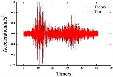
a) Long beam

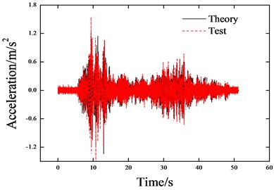
b) Short beam

Results show that: the numerical rules of the theoretical results coincide well with the test results, only the numerical values have a discrepancy. During the simulation analysis, the bearing (high damping rubber bearing) is considered to have linearity, which was not the case in the test. However, this has little effect on the numerical rules. This paper attempted to regulate the bearing stiffness value, and from the simulation results we can see that the wave forms of the acceleration and displacement time interval curves coincide well with each other, only the numerical values have a little discrepancy.

5.2. Effect of track constraint on the beam’s natural vibration frequency

After the test rail’s installation, by once again sweeping the test model at white noise frequency, the natural vibration frequency results for the bridge beams were obtained as shown in Table 6. The results show, that with track constraint, the natural vibration frequencies of the bridge girders are improved. Due to the low longitudinal stiffness of the long beam, the track frame formed of 12 sleepers provided a greater constrained force, and the natural vibration frequency increased by 3.66 Hz. Meanwhile, the longitudinal stiffness of the short beam is relatively larger, and only 6 sleepers provided the longitudinal constraint, the natural vibration frequency increased slightly to approximately 1.06 Hz.

5.3. Beam displacement and rail stress results

The test was conducted by applying seismic waves after the white noise frequency sweep test, as detailed in Table 3.

5.3.1. Beam displacement

Due to a relatively large volume of data, only the beam maximum displacements were extracted, as shown in Table 7.

Table 7Maximum beam displacement (unit: mm)

Case	Long beam			Short beam
	With rail		Without rail theory	With rail		Without rail theory
	Test	Theory		Test	Theory
EL-0.1 g	1.2	0.9	4.2	0.6	0.5	0.8
EL-0.2 g	2.2	1.5	11.1	1.0	0.9	1.5
EL-0.4 g	9.0	4.2	44.8	2.0	1.8	2.9
KB-0.1 g	1.2	0.7	6.7	0.5	0.3	0.6
KB-0.2 g	3.0	2.2	21.8	1.2	0.6	1.4
KB-0.4 g	14.2	3.5	49.0	2.3	1.3	2.6
WC-0.1 g	0.8	0.6	3.8	0.3	0.2	0.5
WC-0.2 g	2.0	1.3	10.2	0.9	0.6	1.4
WC-0.4 g	8.7	3.6	37.4	2.0	1.1	2.3

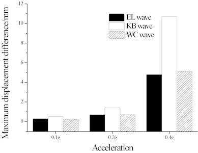
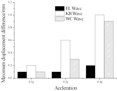
When considering the track constraint, the beam seismic displacement had significantly declined, proving the track restraint is beneficial to bridge seismic resistance. The beam displacement difference between test and theoretical computation is shown in Fig. 9.

According to the test and theoretical results, the test’s maximum beam displacement was greater than theoretical results, and the beam displacement difference between test and theoretical computation is increased with the acceleration.

This is mainly due to the dynamic change in relative displacement between the rail and beam under seismic loading, and ballast bed will be subject to durable dynamic reciprocated changes, which can weaken ballast resistance. Granular railway ballast is characterized by dispersion, composition, and large dimensional differences (Lim, 2004; Indraratna, 2005), the dynamic hysteretic change of the ballast longitudinal resistance is complex and quite different from that of the ideal elasto-plastic hysteretic route. The ballast longitudinal resistance is cyclic and hysteretic under the dynamic seismic excitation load and degenerates cyclically, which makes the test’s beam displacement greater than theoretical results (based on the ideal elasto-plastic hysteretic ballast resistance). Furthermore, the dynamic softening behavior of granular ballast bed is dependent on the exerted acceleration amplitude, the higher the exerted acceleration amplitude, the severer the dynamic softening characteristics. Therefore, the greater the seismic acceleration, the bigger the beam displacement deviation between test and theoretical computation. The assumed ideal elastic-plastic resistance used in theoretical calculations would underestimate the actual displacement; the greater the seismic intensity, the more seriously undervalued the beam displacement becomes.

Fig. 9Test and theoretical beam displacement difference

a) Long beam

b) Short beam

5.3.2. Rail stress test results

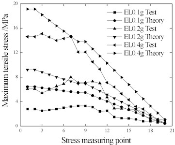
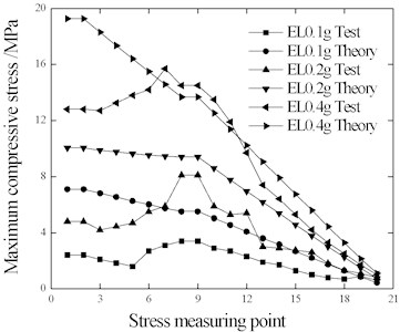
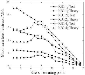
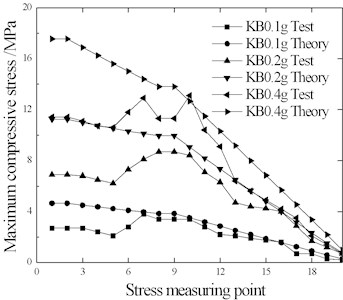
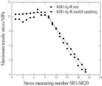
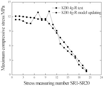
The comparison of rail maximum tensile stress and compressive stress is shown in Figs. 10-12.

With the increase of seismic intensity, the rail stress of each measuring point correspondingly increases significantly. With the exception of a few measuring points with individual conditions (EL-0.4 g and WC-0.4 g), the rail stress test results were lower than the theoretical results. This indicates that the ideal elastic-plastic resistance used in the theoretical calculation overestimates the ballast dynamic longitudinal resistance, which could explain why the test beam displacement is greater than the theoretical value in Table 7.

According to the results obtained based on simulated calculations, the stress of measuring point SR20 close to the free end of the rail is the lowest. The ballast resistance at the sleeper node at any integral time for the simulation model does not change. Therefore, as shown in the figure, all rail stresses from measuring points SR1 to SR20, which are calculated in the simulation, change linearly. All points of the rail with peak stress, which are calculated in the simulation, are selected at the same time. The rail stress decreases linearly, indicating that the long/short beams displace in the same direction; namely the resistances of all sleeper nodes point to the same direction.

Measuring points SR9 to SR20 are set on the long beam, according to the test results, the rail stress decreases between these two points, which coincides with the theoretical results. Meanwhile, the tested stresses of measuring points SR1 to SR8 approximates an increasing trend. This indicates that the displacement results of the long/short beams at time points under peak stresses are opposite, and the ballast resistances and sleeper nodes are also opposite, which does not coincide with the theoretical results. Moreover, the displacement time intervals of the long/short beams shown in Fig. 8 this point, indicating that the stresses of measuring points SR1 to SR8 are far lower than the theoretical values.

Moreover, the track-bridge displacement caused by earthquakes can disturb the ballast bed and influence track resistance, therefore, before and after each excitation test, the structure was scanned with white noise in order to observe the changing natural frequencies of the two beams. The result shows that, by taking EL0.1 g and EL0.4 g as examples, the natural frequencies of the beams decrease after the test, which indicates that the ballast longitudinal resistance decreases under seismic loading. In addition, when the peak maximum acceleration of the seismic wave is low, the overall natural frequencies of the beams will not significantly decrease, however, when the peak acceleration is high, the natural frequencies will show a significant decrease due to a corresponding decrease in natural frequencies along with the increasing relative displacement of the long beam.

Fig. 10Rail stress under EL wave

a) Tensile stress

b) Compressive stress

Fig. 11Rail stress under KB wave

a) Tensile stress

b) Compressive stress

Fig. 12Rail stress under WC wave

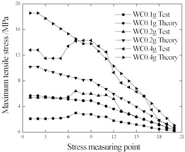
a) Tensile stress

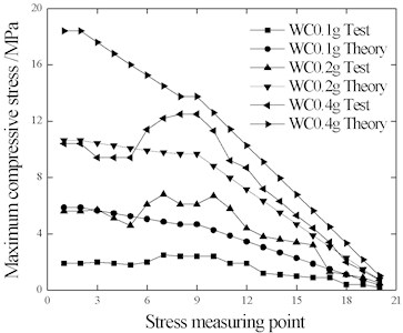
b) Compressive stress

5.3.3. The seismic response of the ballast longitudinal resistance

The theoretical results of the hysteretic force-displacement response of a ballast element near the measuring point SR20 is plotted in Fig. 13. Results show that: the ballast resistance-displacement hysteretic curve coincides well with the ideal elastic-plastic resistance in Fig. 6, and the value of the yielding force is nearly 1.2 kN, which is the maximum force transmissible by a single ballast element.

As mentioned above, ballast beds are subject to a dynamic reciprocating state under seismic loading, the contact relations between the granules will change, wherein some will flow and redistribute. The dynamic hysteretic change of the ballast longitudinal resistance is complex and quite different from that of the ideal elasto-plastic hysteretic route. Therefore, in order to make a comparison with the theoretical results, the test results of the hysteretic force-displacement response of a ballast element is plotted in Fig. 14.

Fig. 13Ballast force-displacement responses

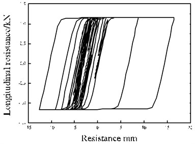
Fig. 14Ballast resistance-displacement hysteretic curve

Fig. 15Bearing capacity degeneration of ballast beds

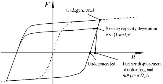
The test results show that granular ballast beds are not ideal elastic bodies due to their microstructure characteristics such as internal pores, intergranular contact and friction. The ballast longitudinal resistance is cyclic and hysteretic under the cyclic excitation of a dynamic seismic load and degenerates cyclically (Fig. 15), influencing the rail longitudinal force value and distribution of CWR on bridges.

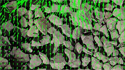
Moreover, the degeration of granular ballast bed under seismic loading is mainly caused by stressed and deformed granules. Images of the ballast surface were taken using a digital camera for observing and measuring ballast movement during the tests. The digital camera was set above the ballast near the beam gap and the image scales were approximately 3.5 pixels per millimeter for the 1,000-mm-wide testing area. Fig. 16 shows the displacement of the ballast grains obtainted by the PIV analyses (Louis, 2014) of the images taken under the the KB-0.2 g case. The technique is capable of providing a clear picture of overall movements, which can reflect the motion law of ballast under seismic loading.

As shown in Fig. 16, the ballast granules move irregularly under seismic loading, wherein they scatter in different directions, some flow and redistribute and the packing state and resistance performance of the ballast bed thus changes. In addition, under seismic loading, ballast grains display insignificant movement compared to the initial loading state and experience obvious overturning and movement changes. The track bed becomes loose and reconstructed. In the hysteretic curve (Fig. 14), the test curve of the granular ballast bed shows dynamic softening properties.

Fig. 16Motion of ballast grains

6.1. Amended model selection

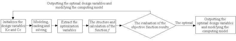
The above results show that the theoretical results for rail stress and beam displacement show large discrepancies with the test results, proving the changing form of ballast longitudinal resistance during the test differs greatly from the ideal elastic-plastic resistance. In this section, the numerical model is amended according to the test results, and the nonlinear resistance elements of equivalent stiffness and equivalent damping are introduced in order to optimize the numerical model of CWR on bridges and make a reasonable selection for their parameters.

For granular ballast beds used under seismic loading, since the dynamic displacement caused by longitudinal excitation can lead to a reciprocating cyclic and hysteretic resistance of ballast beds, such dynamic resistance is in relation to the ballast bed density, ballast material, dynamic displacement frequency and amplitude etc.; the key problem to be solved for theoretical calculation is the reasonable selection of hysteretic curves of the dynamic resistance of ballast beds. Considering the major role of ballast resistance is to restrict the beam displacement and dissipate energy under seismic loading, the equivalent stiffness $K_e$ and equivalent damping $C_e$ are introduced, as shown in Fig. 17. Moreover, these two coefficients can be obtained through the modified finite element model technique [23], and implemented by the optimization module of ANSYS [24], though the specific details of the theory are beyond the scope of this paper.

When using the ANSYS module, the design variables, optimization variables and objective functions, in addition to the range of design variables all need to be determined for model optimization. Three types of variables are adopted for the ANSYS optimization module during the correction and optimization of the model, which are as follows:

1) Design variables (DVs): The design variables of values are subject to change during the analysis. Generally, all design variables should be limited to a certain range.

2) State variables (SVs): Values for restricting the design, which can be independent variables or functions of design variables.

3) Objective function (OBJ): This value is required to be as low as possible, and should be a function of the design variables; that is, the objective function changes with the design variables. Only one objective function is allowed to be defined in practice for optimization and analysis. Common functions are stress, deformation, weight, or the minimum mean value and minimum variance of a result.

Fig. 17Amended model of test structure

The ANSYS optimization module primarily has two optimization modes, which are as follows:

The first is a zero-order optimization method, namely the common function approximation optimization method. Essentially, it aims to fit a solution space through a surface function obtained based on least square method approximation, then calculate the limits, and then establish the maxima and minima of the surface function. It is always adopted for approximate optimization due to low accuracy.

The second optimization method is an upgrade of the first method, namely the first-order optimization method. The first-order partial derivatives of state variables and objective functions to the design variables can be obtained accurately according to a gradient search (conjugate gradient method or the quickest decrease method).

This test focuses on the rail stress and beam displacement measured during seismic excitation. From the test results, it can be seen that during vibration, the reciprocating displacement of the long beam and the axial rail stress within the long/short beam gaps are high. The measured maximum displacement $d{}_{\mathrm{m}\mathrm{a}\mathrm{x}}{}^{\mathrm{}}\mathrm{}$ of the long beam and the maximum axial tensile stress $\sigma {}_{\mathrm{m}\mathrm{a}\mathrm{x}}{}^{\mathrm{}}\mathrm{}$ at measuring point SR9 were adopted as the optimization variables, and the constructed objective functions is the sum of the relative errors of the long beam maximum displacement and rail maximum axial tensile stress at measuring point SR9.

6.2. Example of model amendment

In this section, the KB-0.4 g case in Table 3 is taken as an example to be analyzed.

6.2.3. Steps of model amending

The steps of the model amending analysis and calculation are shown in Fig. 18.

Fig. 18Steps of model modification

6.2.4. Results of model amendment

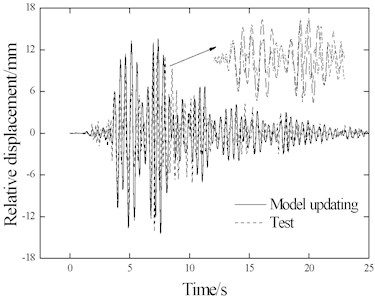
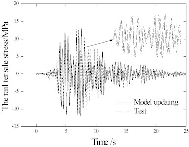
Based on the amended calculation model and combined with the optimization method, the optimal equivalent stiffness coefficient $K_e$ and damping coefficient C_e under case KB-0.4 g were obtained as 69384 N/m and 1090.3 N·S/m, respectively. Comparison of the results of the long beam displacement and rail stress at measuring point S9 are shown in Fig. 19 and Fig. 20.

Fig. 19Displacement and stress comparison

a) Long beam displacement

b) Stress at measuring point S9

As shown in Fig. 19 and Fig. 20, the peak value and frequency of the theoretical results coincide well with those of the test results. As shown in the close-up view of the measuring points in Fig. 15, the wave forms of the rail stress and beam displacement time interval curves also coincide well with each other. The stress values and distribution of all measuring points on the rail coincide well with the test results, indicating the equivalent stiffness ($K_e$ and $C_e$) of the ballast obtained based on the optimization method can help to obtain test results through calculation of the simulation.

In regards to existing research, the related issues are always analyzed based on the ideal elastic-plastic longitudinal resistance of ballast. This hypothesis has been proved innacurate according to the test results of this paper. Moreover, based on the test results, a theoretical method, which is more applicable in obtaining practical results, is presented through model correction. The new theoretical calculations obtained from the modified finite element model coincide well with the test results.

Fig. 20Rail stress comparison

a) Tensile stress

b) Compressive stress