Investigation the influence of shear distortion, rotary inertia and longitudinal vibration on the power flow transmission of a finite L-shaped beam

Li, Jia-Xing; Zhu, Xue-Zhi; Chen, Zhao-Bo; Jiao, Ying-Hou

doi:10.21595/jve.2017.17850

Journal of Vibroengineering

Browse Journal

Submit article

Published: 30 June 2017

Check for updates

Investigation the influence of shear distortion, rotary inertia and longitudinal vibration on the power flow transmission of a finite L-shaped beam

Jia-Xing Li¹

Xue-Zhi Zhu²

Zhao-Bo Chen³

Ying-Hou Jiao⁴

^{1, 2, 3, 4}Harbin Institute of Technology, Harbin, China

Corresponding Author:

Jia-Xing Li

Cite the article Download PDF

Downloads 1714

WoS Core Citations 2

CrossRef Citations 1

Abstract

The dynamics response and power flow propagation in the L-shaped beam with finite dimension were investigated. A L-shaped beam dynamic model was established on the basis of Timoshenko beam theory (TBT) and Euler-Bernoulli beam theory (EBT). The analytical solution was obtained and the beam flexural and longitudinal motion was described by using the traveling wave approach. The effects of shear distortion and rotary inertia on the total power flow and its components were examined. Results shown that the structure resonant frequencies are obviously affected by the shear distortion and rotary inertia, especially for the medium and high frequency ranges. The power flow amplitude is obviously increased on the premise of considering the longitudinal vibration. Consequently, the longitudinal vibration should be considered for the power flow and its components in the L-shaped beam.

1. Introduction

Finite L-shaped beams are usually encountered in engineering device and structure, such as the ship hull, aircraft fuselages and satellite structures. For example, the deployable truss structure and the camera support structure of satellites are a kind of girder structure which usually is modeled as a finite L-shaped beam. Vibration energy is introduced by external force excitation, such as the reaction flywheel in satellite and the engine rotor of ship, which can induce the whole structure vibration. However, the vibration energy propagating through the finite beam structures is mostly investigated by the Euler-Bernoulli beam theory (EBT) and the influence of longitudinal vibration is seldom discussed. Further, the shear distortion and rotary inertia are excluded in the EBT, which would result in misestimating the natural frequencies of L-shaped beam structure. Fortunately, the Timoshenko beam theory (TBT) is available to research the vibratory power flow propagation in the finite L-shaped beam.

Many research papers have been published about the vibration propagation and power flow of the beam and plate structures. Zhao et al. studied the disturbance propagation and active vibration control in complex space truss structures based on advanced Timoshenko theory using traveling wave approach. The numerical results indicate that dynamic responses are more accurate using the Timoshenko beam model, especially for the medium and high frequency ranges [1]. Mei studied the active control of coupled bending and axial vibrations in L-shaped and portal planar frame structures using traveling wave approach. Both Euler-Bernoulli and Timoshenko bending theory were used to modeling and controlling the flexural vibrations in planar frames. The numerical results shown that the rotary inertia and shear distortion should be taken into account for the higher frequencies, especially for transverse dimensions are not negligible with respect to the wavelength [2]. Lin presented the analytical solution for the vibration response of ribbed plate with all boundary clamped by using traveling wave method, and the ribbed plate experimental investigation provided verification results to the analytical solution [3]. Kang and Riedel presented the coupling effects of three elastic wave modes (flexural, tangential, and radial shear) on the dynamics of a planar curved beam. The contributions of the dynamic and high-order elastic coupling terms to the response of a thick curved beam are quite significant. Therefore, the coupling terms should not be neglected for an accurate analysis of a thick curved beam with a large curvature parameter [4].

The disturbance propagation and active vibration control of a finite L-shaped beam was studied by using the traveling wave approach based on Euler-Bernoulli theory. The calculation results indicate that the dynamics responses calculated by traveling method are more precise than those by FEM model [5]. Mei studied the active control of bending vibrations in beams by using the hybrid approach based on the advanced Timoshenko theory. He found that the hybrid approach has better broadband active vibration control performance than that of modal or wave control alone [6]. Sniady studied the dynamical response of a finite Timoshenko beam excited by a constant velocity moving force with simply support boundary conditions [7]. Mei analyzed the in-plane vibration of H- and T-shaped planar frame structures by using the wave vibration approach based on Timoshenko beam theory. He found the effects of rotary inertia and shear distortion become important at higher frequencies and the types of external excitations not change the structure resonance frequencies [8]. Using a developed analytical method which included the rigid and nonrigid connectors of practical interest, Li et al. investigated the vibrations and power flow between two-coupled beams with elastically restrained boundary conditions. Results revealed that the current method has excellent agreement with the FEA solution and can extend to more complex structures or systems composed of beams [9].

Audrain investigated the finite beam with piezoelectric patch control actuator and accelerometer probe error sensors for structural intensity. They found that the structure intensity control is more effective than the acceleration control, and the intensity control allows the error sensors to placed closer to the control source and the disturbance, while preserving a good control performance [10]. Kessissoglou presented the power flow propagation in the L-shaped plates and the effects of in-plane waves on the power flow are analyzed by the combination of the modal method and the traveling wave method. Numerical simulations show that the in-plane waves raise total power at the structural resonances and the effect increases as the frequency increases [11]. Carvalho and Zindeluk investigated the active control of waves in the Timoshenko beams using forces or moment pairs [12]. Patrice et al. analyzed the instantaneous structure intensity active control of a beam covered with piezoelectric patch (the control source) and piezoelectric strain sensors (PVDF) by using theoretical and experimental approaches. They found that this control approach can achieve a high attenuation for controlling the harmonic disturbance [13].

In the present investigation, the dynamics response and power flow propagation of a finite L-shaped beam under a concentrate external force were studied by EBT and TBT. The traveling wave approach is utilized to calculate the dynamics response and power flow of the finite L-shaped beam. The power flow is presented in the spectrum form. The power flow results are calculated by the EBT and TBT for investigation the influence of shear distortion and rotary inertia. Moreover, the influence of the longitudinal vibration on the power flow and the components in high frequency range were studied too.

2. Flexural and longitudinal vibration of Timoshenko coupled beams

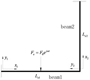
The geometric model of a finite L-shaped beam and the coordinate system are presented in Fig. 1. The L-shaped beam is clamped at the boundary edges corresponding to $x_{1} =$ 0 and $x_{2} = L_{x 2}$ . The junction corner of the two beams corresponding to $x_{1} = L_{x 1}$ and $x_{2} =$ 0. The two beams have the same material, thickness and width for mathematical simplicity. The Euler-Bernoulli beam theory and Timoshenko beam theory are used to investigate the influence of beam shear distortion and rotary inertia on the power flow in the beam structure.

The EBT model considers the lateral inertia and elastic forces caused by transverse bending deflection, that is, the effects of rotary inertia and shear distortion are neglected. The difference between EBT and TBT is that the latter includes the effects of rotary inertia of mass and the shear distortion, which is important when the transverse dimensions are not negligible with respect to the wavelength. The governing equation of the bending and slop displacement of Timoshenko beam for the external forces can be expressed as follows [2, 6]:

1

G A κ [\frac{\partial ψ (x, t)}{\partial x} - \frac{\partial^{2} w (x, t)}{\partial x^{2}}] + ρ A \frac{\partial^{2} w (x, t)}{\partial t^{2}} = f (x, t),

2

E I \frac{\partial^{2} ψ (x, t)}{\partial x^{2}} + G A κ [\frac{\partial w (x, t)}{\partial x} - ψ (x, t)] - ρ I \frac{\partial^{2} ψ (x, t)}{\partial t^{2}} = 0,

where $x$ is the position along the beam axis, $t$ the time, $w$ the transverse displacement of the center line of the beam, $I$ the area moment of inertia of beam cross section, $A$ the beam cross-section area, $ρ$ the material density, $E$ the Young’s modulus, $G = E / [2 (1 + μ)]$ the shear modulus, $μ$ the Poission’s ratio, $κ$ the Timoshenko shear factor, $ψ$ the slope due to bending, and $f (x, t)$ the externally applied force.

Fig. 1Geometrical description and coordinate system for the L-shaped beam

By employing the traveling wave approach, the transverse displacement and shear slope of the finite beam can be written as [6]:

3

w (x, ω) = C_{1} (ω) e^{j k_{n 1} x} + C_{2} (ω) e^{k_{n 2} x} + C_{3} (ω) e^{- j k_{n 1} x} + C_{4} (ω) e^{- k_{n 2} x},

4

ψ (x, ω) = j P_{n} C_{1} (ω) e^{j k_{n 1} x} + N_{n} C_{2} (ω) e^{k_{n 2} x} - j P_{n} C_{3} (ω) e^{- j k_{n 1} x} - N_{n} C_{4} (ω) e^{- k_{n 2} x},

where:

5

P_{n} = k_{n 1} (1 - \frac{ω_{n}^{2}}{k_{n 1}^{2} C_{s}^{2}}), N_{n} = k_{n 2} (1 + \frac{ω_{n}^{2}}{k_{n 2}^{2} C_{s}^{2}}),

6

k_{n 1} = {\{\frac{1}{2} [{(\frac{1}{C_{s}})}^{2} + {(\frac{C_{r}}{C_{b}})}^{2}] ω_{n}^{2} + \sqrt{\frac{ω_{n}^{2}}{C_{b}^{2}} + \frac{1}{4} {[{(\frac{1}{C_{s}})}^{2} - {(\frac{C_{r}}{C_{b}})}^{2}]}^{2} ω_{n}^{4}}\}}^{1 / 2},

7

k_{n 2} = {\{|\frac{1}{2} [{(\frac{1}{C_{s}})}^{2} + {(\frac{C_{r}}{C_{b}})}^{2}] ω_{n}^{2} - \sqrt{\frac{ω_{n}^{2}}{C_{b}^{2}} + \frac{1}{4} {[{(\frac{1}{C_{s}})}^{2} - {(\frac{C_{r}}{C_{b}})}^{2}]}^{2} ω_{n}^{4}}|\}}^{1 / 2},

8

C_{b} = \sqrt{\frac{E I}{ρ A}}, C_{s} = \sqrt{\frac{G A κ}{ρ A}}, C_{r} = \sqrt{\frac{ρ I}{ρ A}} .

The unknown wave amplitude $C_{i} (ω)$ for $i =$ 1,…, 4 can be obtained with the given boundary conditions. For the finite rod longitudinal vibration, the quasi-longitudinal wave solution can be obtained by the travelling wave approach, which can be written as [5]:

9

u (x, ω) = B_{1} (ω) e^{j k_{L} x} + B_{2} (ω) e^{- j k_{L} x},

where $k_{L} = ω \sqrt{ρ A} / \sqrt{E}$ is the quasi-longitudinal wave number, and $B_{1} (ω)$ and $B_{2} (ω)$ the unknown wave displacement amplitudes, which can be determined by the boundary condition. The beam vibration information of the transverse and longitudinal disturbance is represented by Eqs. (3), (4) and (9). Once these unknown wave displacement amplitudes are obtained, the beam dynamic response can be calculated. The dynamics response of beam structures can be calculated by combining the travelling approach and substructure approach. Therefore, the travelling approach and substructure approach are employed to calculate the dynamic response of the L-shaped beam.

The external force location can be treated as the continuous condition. The governing equations of the flexural and longitudinal displacement in beam 1 can be written as:

10

w_{1 Ι} (x_{1}, ω) = C_{1} (ω) e^{j k_{n 1} x_{1}} + C_{2} (ω) e^{k_{n 2} x_{1}} + C_{3} (ω) e^{- j k_{n 1} x_{1}} + C_{4} (ω) e^{- k_{n 2} x_{1}}, x_{1} \leq x_{0},

11

ψ_{1 Ι} (x_{1}, ω) = j P_{n} C_{1} (ω) e^{j k_{n 1} x_{1}} + N_{n} C_{2} (ω) e^{k_{n 2} x_{1}}

- j P_{n} C_{3} (ω) e^{- j k_{n 1} x_{1}} - N_{n} C_{4} (ω) e^{- k_{n 2} x_{1}},

12

w_{1 Ι Ι} (x_{1}, ω) = C_{5} (ω) e^{j k_{n 1} x_{1}} + C_{6} (ω) e^{k_{n 2} x_{1}} + C_{7} (ω) e^{- j k_{n 1} x_{1}} + C_{8} (ω) e^{- k_{n 2} x_{1}},

x_{0} < x_{1} \leq L_{x 1},

13

ψ_{1 Ι Ι} (x_{1}, ω) = j P_{n} C_{5} (ω) e^{j k_{n 1} x_{1}} + N_{n} C_{6} (ω) e^{k_{n 2} x_{1}}

- j P_{n} C_{7} (ω) e^{- j k_{n 1} x_{1}} - N_{n} C_{8} (ω) e^{- k_{n 2} x_{1}},

14

u_{1} (x_{1}, ω) = B_{1} (ω) e^{j k_{L} x_{1}} + B_{2} (ω) e^{- j k_{L} x_{1}} .

The governing equations of flexural and longitudinal displacement in beam 2 can be written as:

15

w_{2} (x_{2}, ω) = C_{9} (ω) e^{j k_{n 1} x_{2}} + C_{10} (ω) e^{k_{n 2} x_{2}} + C_{11} (ω) e^{- j k_{n 1} x_{2}} + C_{12} (ω) e^{- k_{n 2} x_{2}},

16

ψ_{2} (x_{2}, ω) = j P_{n} C_{9} (ω) e^{j k_{n 1} x_{2}} + N_{n} C_{10} (ω) e^{k_{n 2} x_{2}}

- j P_{n} C_{11} (ω) e^{- j k_{n 1} x_{2}} - N_{n} C_{12} (ω) e^{- k_{n 2} x_{2}},

17

u_{2} (x_{2}, ω) = B_{3} (ω) e^{j k_{L} x_{2}} + B_{4} (ω) e^{- j k_{L} x_{2}} .

There sixteen unknown flexural, shear slope and longitudinal wave displacement amplitudes corresponding to $C_{i} (ω)$ for $i =$ 1,…, 12 and $B_{a} (ω)$ for $a =$ 1,…, 4. Sixteen equations could be developed from the boundary conditions at the clamped edges, continuity conditions at the external point force location and coupling conditions at the corner junction of the two beams of the L-shaped beam structure. The six boundary conditions at the clamped edges can be written as:

18

{w_{1 Ι} (x_{1}, ω)|}_{x_{1} = 0} = {w_{2} (x_{2}, ω)|}_{x_{2} = L_{x 2}} = 0,

19

{u_{1} (x_{1}, ω)|}_{x_{1} = 0} = {u_{2} (x_{2}, ω)|}_{x_{2} = L_{x 2}} = 0,

20

{ψ_{1 Ι} (x_{1}, ω)|}_{x_{1} = 0} = {ψ_{2} (x_{2}, ω)|}_{x_{2} = L_{x 2}} = 0 .

There are four continuity conditions at the external force location, the continuous equations at the beam 1 can be written as:

21

{w_{1 Ι} (x_{1}, ω)|}_{x_{1} = x_{0}} = {w_{1 Ι Ι} (x_{1}, ω)|}_{x_{1} = x_{0}}, {ψ_{1 Ι} (x_{1}, ω)|}_{x_{1} = 0} = {ψ_{1 Ι Ι} (x_{1}, ω)|}_{x_{1} = x_{0}},

22

{\frac{\partial ψ_{1 Ι} (x_{1}, ω)}{\partial x}|}_{x_{1} = x_{0}} = {\frac{\partial ψ_{1 Ι Ι} (x_{1}, ω)}{\partial x}|}_{x_{1} = x_{0}},

23

{[\frac{\partial w_{1 Ι} (x_{0}, ω)}{\partial x} - ψ_{1 Ι} (x_{0}, ω)]|}_{x_{1} = x_{0}} - {[\frac{\partial w_{1 Ι Ι} (x_{0}, ω)}{\partial x} - ψ_{1 Ι Ι} (x_{0}, ω)]|}_{x_{1} = x_{0}} = - \frac{F_{0}}{G A κ} .

Finally, there are six continuity equations at the coupling junction of two beams corresponding to $x_{1} = L_{x 1}$ and $x_{2} =$ 0. The coupling equations at the junction place of two beams can be written as:

24

{w_{1 Ι Ι} (x_{1}, ω)|}_{x_{1} = L_{x 1}} = {u_{2} (x_{2}, ω)|}_{x_{2} = 0}, {w_{2} (x_{2}, ω)|}_{x_{2} = 0} = {- u_{1} (x_{1}, ω)|}_{x_{1} = L_{x 1}},

25

{ψ_{1 Ι Ι} (x_{1}, ω)|}_{x_{1} = L_{x 1}} = {ψ_{2} (x_{2}, ω)|}_{x_{2} = 0}, {M_{x 1 Ι Ι} (x_{1}, ω)|}_{x_{1} = L_{x 1}} = {M_{x 2} (x_{2}, ω)|}_{x_{2} = 0},

26

{Q_{x 1 Ι Ι} (x_{1}, ω)|}_{x_{1} = L_{x 1}} = {N_{x x 2} (x_{2}, ω)|}_{x_{2} = 0}, {Q_{x 2} (x_{2}, ω)|}_{x_{2} = 0} = {- N_{x x 1} (x_{1}, ω)|}_{x_{1} = L_{x 1}},

where $M_{x}$ is the bending moment, $N_{x}$ is the longitudinal force, $Q_{x}$ is the transverse shear force. The expression of $M_{x}$ , $N_{x}$ and $Q_{x}$ can be written as [2, 5, 6]:

27

M_{x} = - E I \frac{\partial ψ}{\partial x}, N_{x} = E A \frac{\partial u}{\partial x}, Q_{x} = - G A κ [- ψ + \frac{\partial w}{\partial x}] .

Using the sixteen developed equation, a matrix expression can be obtained as $[β] X = F$ , where $[β]$ is a 16×16 matrix. $X$ and $F$ are the wave amplitude coefficients and force matrices, respectively, and are given by:

28

X = {\{C_{1}, \dots, C_{12}, B_{1}, B_{2}, B_{3}, B_{4}\}}^{T},

29

F = {\{0,0, 0,0, 0,0, 0, \frac{F_{0}}{G A κ}, 0,0, 0,0, 0,0, 0,0\}}^{T} .

Solutions to the unknown wave amplitude coefficients in Eqs. (16) to (17) can be solved by $X = {[β]}^{- 1} F$ .

3. Flexural vibration only of Timoshenko coupled beams

The power flow without considering the longitudinal vibration is calculated to investigate the influence of the longitudinal vibration. The longitudinal force and displacement have been taken into account at the coupling junction of the two beams, when equating the displacements and forces at the junction. The analysis has been reduced to consider only the flexural vibration in the beams, as described in Eqs. (10-13), (15) and (16). For the L-shaped beam without longitudinal vibration, there are only twelve unknown wave amplitude coefficients $C_{i}$ for $i =$ 1,…, 12. At the boundary edges, the boundary conditions have reduced to four, as described by Eqs. (18) and (20). The continuous conditions at the external point force location in beam 1 are unchanged. However, there are only four continuous coupling equations at the junction place of the two beams. The first and second equations are the continuity of moment and slope from beam 1 and beam 2, as described by Eq. (25). The last two equations are deduced by equating the displacements and forces at the corner junction. In this condition, the general expression for the longitudinal waves of the two beams can be written as:

30

u_{1} (x_{1}, ω) = H_{1} (ω) e^{j k_{L} x_{1}}, u_{2} (x_{2}, ω) = H_{2} (ω) e^{- j k_{L} x_{2}},

where $u_{1}$ is the reflected longitudinal wave in beam 1 due to the flexural wave in beam 2, $u_{2}$ is the transmitted longitudinal wave in beam 2 due to the flexural wave in beam 1 impinging on the corner junction. The displacement and force can be simplified by using the Eqs. (24) and (26), and the simplified continuous coupling equations can be written as:

31

G A κ [- ψ_{1 Ι Ι} (x_{1}, ω) + \frac{\partial w_{1 Ι Ι} (x_{1}, ω)}{\partial x}] = E A j k_{L} w_{1 Ι Ι} (x_{1}, ω),

32

- G A κ [- ψ_{2} (x_{2}, ω) + \frac{\partial w_{2} (x_{2}, ω)}{\partial x}] = E A j k_{L} w_{2} (x_{2}, ω) .

The twelve unknown wave amplitude coefficients can also be solved by using the similar matrix expression $[β] X = F$ . For this case, the matrix $[β]$ is a 12×12, and the wave amplitude coefficients and force matrices are given by:

33

X = {\{C_{1}, C_{2}, \dots, C_{12}\}}^{T},

34

F = {\{0,0, 0,0, 0,0, 0, \frac{F_{0}}{G A κ}, 0,0, 0,0,\}}^{T} .

4. Vibratory power flow in the finite L-shaped beam

The vibratory power flow transmission through beam cross section has three parts. The first one is the shear force power flow, the second one is the bending moment power flow and the last one is the longitudinal force power flow. The instantaneous power flow (time averaged vibration intensity) propagation through the cross section including the longitudinal vibration components can be written as:

35

P_{x} = - [{(j ω w (x, ω))}^{*} Q_{x} (x, ω) - {(j ω ψ)}^{*} M_{x} (x, ω) + {(j ω u (x, ω))}^{*} N_{x} (x, ω)] .

The time averaged vibratory power flow can be expressed as:

36

P_{x a} = - R e [{(j ω w (x, ω))}^{*} Q_{x} (x, ω) - {(j ω ψ)}^{*} M_{x} (x, ω) + {(j ω u (x, ω))}^{*} N_{x} (x, ω)] .

When the beam longitudinal vibration is neglected in the analysis, the above vibratory power flow expression simply reduces to:

37

P_{x} = - [{(j ω w (x, ω))}^{*} Q_{x} (x, ω) - {(j ω ψ)}^{*} M_{x} (x, ω)],

38

P_{x a} = - R e [{(j ω w (x, ω))}^{*} Q_{x} (x, ω) - {(j ω ψ)}^{*} M_{x} (x, ω)] .

5. Numerical simulation and discussion

The L-shaped beam shown in Fig. 1 is computed using travelling wave and substructure method. The material properties of the L-shaped beam are presented as follows: $ν =$ 0.3, $ρ =$ 7800 kg/m³, $E =$ 2.0×10¹¹Pa. The beam structure damping is introduced in the analysis by using the form of complex Young’s modulus $E (1 + j η)$ , where $η =$ 0.001 is the structural loss factor. For the L-shaped beam structure, the two beams have the same crossing section. The width of the beam is $b =$ 0.02 m, and the height of the beam is $h =$ 0.02 m without specification. The lengths of the L-shaped beam are $L_{x 1} =$ 1.2 m and $L_{x 2} =$ 1.0 m respectively. The external point force is located at $x_{0} =$ 0.6 m of the beam 1, and $F =$ 1 N in calculation.

In order to confirm the wave method and the effect of element number of FEM (finite element method) modal, the dynamics response of beam 2 was calculated by MSC/NASTRAN and wave method. The beam 2 of L-shaped beam has been meshed with 40 elements and 160 elements in the FEM model. The spectrum curves are plotted in Fig. 2. As shown in Fig. 2, the results of FEM and travelling wave was found to have good internal consistency in the low frequency range. However, the difference between FEM and wave method arises as the excitation frequency increase, and the difference is clear when the frequency increased.

Besides, the FEM results are convergent to the wave method result when the element number of the FEM model increase. This is because of the uncertainty and the truncation error of the high-order modes in the FEM model. That is, the FEM is not as precise as the wave method for the media and higher frequency rang even though the FEM model employs more elements. The FEM is numerical method and the result is very sensitive to the element number, and the resonant frequencies are different with different element number even in the low frequency range. Consequently, the structure must be meshed refinement in the high frequency range, which will result in excessive degrees of freedom and decrease the computational feasibility [11]. Differently, the travelling wave method is analytical solution and the results stability not changes as the frequency increase. Further, the wave method is suitable for calculating the whole frequency range response and there is no modal restriction. Therefore, the wave method is more suitable for the beam dynamics response analysis especially in the medium and high frequency range.

The transverse displacement response in the beam 1 of L-shaped beam was calculated by TBT and EBT and the response location at $x_{1} =$ 0.6 m, as presented in Fig. 4. The flexural displacement of single beam at location $x =$ 0.6 m is shown in Fig. 4. The boundary conditions and dimension of the single beam are the same as the beam 1 of the L-shaped beam in Fig. 3. The displacement spectrum plots reveal that the results calculated by TBT and EBT are obvious different. The natural frequencies by TBT and EBT are coincidence with each other well in the lower frequency range.

Fig. 2Displacement response comparison at x2= 0.5 m of the beam 2 between FEM and wave method

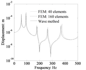
Fig. 3Displacement response comparison of L-shaped beam calculated by TBT and EBT

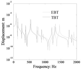
Fig. 4Displacement response comparison of a single beam calculated by TBT and EBT

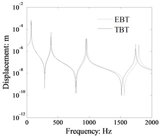
However, the resonant frequencies are different as the excitation frequency increase. The natural frequencies obtained by TBT are obvious lower than those by EBT in high frequency rang. The phenomenon reason is that the beam shear distortion is not taken into account in the EBT, therefore the beam shear rigidity becomes infinite in the Euler-Bernoulli beam theory. Thus, the natural frequencies of Euler-Bernoulli beam are misestimated by the EBT. The influence of shear rigidity on the natural frequency of a beam can be neglected in the lower frequency rang. The shear rigidity of Timoshenko beam model is lower than that of Euler-Bernoulli beam model for the shear distortion and rotary inertia are taken into account in the TBT. Finally, the resonant frequencies calculated by TBT are lower than those by EBT, especially in higher frequency rang. The results indicate that the dynamic response should be calculated by TBT for TBT is more accurate than EBT.

From the displacement spectrum curves plotted in Fig. 3, the resonant peak number is obviously more different between TBT and EBT than that shown in Fig. 4. The reason is that the L-shaped beam structure includes the coupled beam 2, which will increase the structure natural frequencies number and enlarge the effect of shear distortion and rotary inertia. Therefore, the coupled effect of the beams in the L-shaped beam should be taken into account in the study of the dynamic response of each beam.

The power flow results in beam 1 calculated by TBT and EBT with different height are plotted in Figs. 5 to 7 (the response location at $x =$ 0.9 m). From the results presented in Fig. 5, we can see that the spectrum curve of power flow calculated by TBT is consistent with that by EBT from the initial frequency range. However, the natural frequencies by TBT and EBT become different as the excitation frequency increase and the difference becomes more obvious in the medium and higher frequency range. As shown in Fig. 6, the difference of power flow by TBT and EBT are smaller and the resonant peak numbers are much denser than those in Fig. 5. The power flow spectrum results in Fig. 7 reveal that the natural frequencies by TBT and EBT are closer in the medium and higher frequency rang as the beam height decrease, and the resonant peaks are much denser compare to Figs. 5 and 6. This is because the beam cross section height is smaller than those in Figs. 5 and 6. The power flow results indicate that the shear distortion and rotary inertia will introduce obvious influence on the natural frequencies of L-shaped beam especially in the medium and higher frequency rang. The influence of shear distortion and rotary inertia will become more obvious as the beam cross section height increasing.

Fig. 5Comparison power flow in the beam 1 of the L-shaped beam calculated by TBT and EBT (cross-section: 0.03 m×0.03 m, dB ref: 10-12 W)

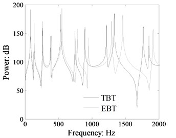
Fig. 6Comparison power flow in the beam 1 of the L-shaped beam calculated by TBT and EBT (cross-section: 0.03 m×0.01 m, dB ref: 10-12 W)

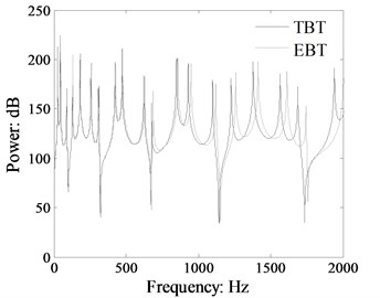
Fig. 7Comparison power flow in the beam 1 of the L-shaped beam calculated by TBT and EBT (cross-section: 0.03 m×0.005 m, dB ref: 10-12 W)

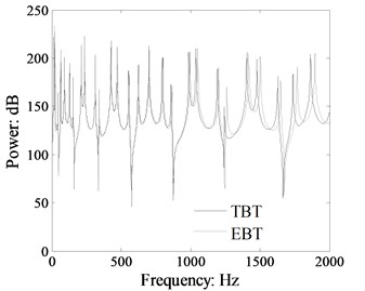
Fig. 8Comparison longitudinal force power flow in the beam 1 of the L-shaped beam calculated by TBT and EBT (cross-section: 0.03 m×0.03 m, dB ref: 10-12 W)

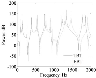
The longitudinal force power flow, transverse force power flow and moment power flow spectrum curves by TBT and EBT are presented in Figs. 8 to 10 (the response location at $x =$ 0.9 m). The power flow spectrum curves shown in Figs. 8-10 give out that the transverse force power flow, moment power flow and the longitudinal force power flow are also obviously affected by the shear distortion and rotary inertia, and the influence law is the same as that depicted in Fig. 5. The results in Figs. 8-10 indicate that the shear distortion and rotary inertia will introduce obvious influence on the power flow components for the medium and higher frequency range, and the higher the frequency is the more obvious the influence is.

Fig. 9Comparison transverse force power flow in the beam 1 of the L-shaped beam calculated by TBT and EBT (crossing section: 0.03 m×0.03 m, dB ref: 10-12 W)

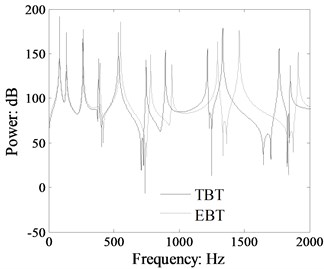
Fig. 10Comparison moment power flow in the beam 1 of the L-shaped beam calculated by TBT and EBT (crossing section: 0.03 m×0.03 m, dB ref: 10-12 W)

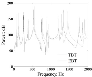
Fig. 11Comparison power flow in the beam 1 of the L-shaped beam with and without longitudinal vibration calculated by TBT (crossing section: 0.03 m×0.03 m, dB ref: 10-12 W)

Comparison power flow in the beam 1 of the L-shaped beam with and without longitudinal vibration calculated by TBT (crossing section: 0.03 m×0.03 m, dB ref: 10-12 W)

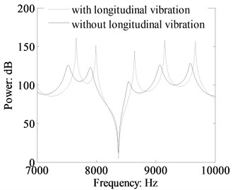
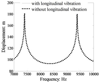
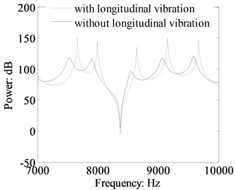
Fig. 12Comparison power flow in a single beam with and without longitudinal vibration calculated by TBT (crossing section: 0.03 m×0.03 m, dB ref: 10-12 W)

In order to investigate the effect of beam longitudinal vibration on the vibratory power flow in the beam structure, the vibratory power flow with and without the longitudinal vibration in the beam 2 of L-shaped beam and a single beam are plotted in Figs. 11 and 12. The single beam dimension and material property are the same with the L-shaped beam. From the results shown in Fig. 11, we can see that the vibratory power flow is obviously affected by the longitudinal vibration. At the resonant peaks and the nearby region, the power flow is increased remarkably under the consideration of the longitudinal vibration. The beam longitudinal wave length is close to the flexural wave length as the excitation frequency increasing, which result in the longitudinal wave ingredient of vibratory power flow becomes obviously in the in the high frequency range. The flexural wave impinging the corner junction will induce longitudinal wave in the connected beam and the longitudinal wave can transform into flexural wave as it travels through the corner junction. In high frequency range, the phenomenon becomes more obviously for the approximative wave length of longitudinal and flexural wave.

It can be seen form Fig. 12 that the vibratory power flow curves are uniform regardless of the longitudinal vibration include or not. This is due to the flexural and longitudinal vibrations are independent with each other in the single beam. Therefore, the coupling and transformation between flexural and longitudinal vibration only appear in the beam connection point. The results indicate that the beam longitudinal vibration should be taken into account when calculating the beam connection structure vibratory power flow for obtaining more accurate analytical results. The influence of longitudinal vibration can be neglected on the condition there is no connection point in the beam structure.

Fig. 13Power flow in the beam 1 and the contribution from the longitudinal and bending vibration calculated by TBT (cross-section: 0.03 m×0.03 m, dB ref: 10-12 W)

Power flow in the beam 1 and the contribution from the longitudinal and bending vibration calculated by TBT (cross-section: 0.03 m×0.03 m, dB ref: 10-12 W)

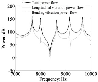
Fig. 14Comparison of the total power flow, bending vibration power flow and longitudinal power flow at the resonant frequencies by TBT (cross-section: 0.03 m×0.03 m, dB ref: 10-12 W)

Comparison of the total power flow, bending vibration power flow and longitudinal power flow at the resonant frequencies by TBT (cross-section: 0.03 m×0.03 m, dB ref: 10-12 W)

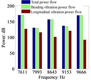
Fig. 15Comparison of the transverse force power flow in the beam 1 with and without longitudinal vibration calculated by TBT (cross-section: 0.03 m×0.03 m, dB ref: 10-12 W)

Comparison of the transverse force power flow in the beam 1 with and without longitudinal vibration calculated by TBT (cross-section: 0.03 m×0.03 m, dB ref: 10-12 W)

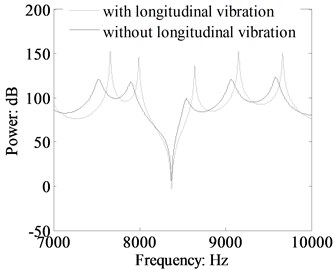
Fig. 16Comparison of the moment power flow in the beam 1 with and without longitudinal vibration calculated by TBT (crossing section: 0.03 m×0.03 m, dB ref: 10-12 W)

Comparison of the moment power flow in the beam 1 with and without longitudinal vibration calculated by TBT (crossing section: 0.03 m×0.03 m, dB ref: 10-12 W)

For obtaining more meticulous observation into the increase in the L-shaped beam power flow when the longitudinal vibration is included, the contribution of the longitudinal vibration to the total power flow, transverse force power flow and moment power flow are presented in Figs. 13 to 16. Fig. 13 shown the total power flow and the bending and longitudinal vibration power flow components in the high frequency range (response location at $x =$ 0.5 m in beam 2). The results in Fig. 13 depict that the longitudinal vibration modes can increase the total power flow at several resonant frequencies. The Fig. 14 indicates that the total power at 7993 Hz and 9153 Hz are obviously increased under consideration the longitudinal vibration. The influence of longitudinal vibration on the total power flow at the other resonant frequencies can be neglected. The main body of the total power flow is the bending vibration component. Figs. 15 and 16 presented the comparison results of transverse force and moment power flow when the longitudinal vibration is included or not. The spectrum curves give out that not only the resonant peak amplitude of total power flow obviously increased, but also the transverse force and moment components on the condition the longitudinal vibration is included. This is due to the longitudinal mode offers an addition path for the flexural vibration energy, and the flexural and longitudinal vibration transform into each other when transmission through the beam corner junction.

6. Experiment arrangement and results discussion

For verifying the dynamic responses and power flow calculated by TBT are more accurate than those by EBT, the cantilever beam vibration experiment is designed for measuring the acceleration response and comparing the testing results with those obtained by TBT and EBT. The experiment rig used in this paper investigation is shown in Fig. 17. The length of the cantilever beam after being clamped on the steel base are measured as $L_{x} =$ 0.42 m and the cross-section dimensions are $h_{b} =$ 0.0075 m and $w_{b} =$ 0.028 m. The cantilever beam is made of aluminum, the material properties of the beam are assumed to be: $E =$ 42×10⁹ Pa, $ρ =$ 2700 kg/m³ and $μ =$ 0.3 in the theory calculation. The instruments used in the experiment include: Lab shop testing system (B&K); a twelve-channel data acquisition equipment (DAE B&K type 3560-D); two accelerometers (B&K type 4507); an Impact Hammer (B&K type 8206-002).

Fig. 17Illustration of the test-rig in the experiment

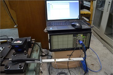
Fig. 18Theory and measured acceleration response of cantilever beam, x1= 0.105 m

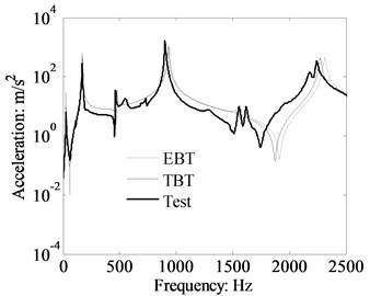
Fig. 19Theory and measured acceleration response of cantilever beam, x2= 0.315 m

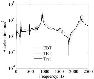
In this experiment investigation, the impact hammer was applied at $x_{0} =$ 0.21 m. The measured acceleration results of the cantilever beam together with those calculated from the analytical results are plotted in Figs. 18 and 19. The theory acceleration curves presented in Figs. 18 and 19 are calculated by TBT and EBT respectively, and the response locations are $x_{1} =$ 0.105 m and $x_{2} =$ 0.315 m. The acceleration spectrum plots in Figs. 18 and 19 reveals that a good agreement has been found between the theory and measured results in the initial testing frequency range. However, the difference has been observed as the frequency increasing. The discrepancy between measured and TBT results is mainly due to the material property of the cantilever beam and the precision accuracy of testing environment in the experiment. The dynamics response also shown that the difference between measured and EBT results become more obvious than that between experiment and TBT as the frequency increasing. For the influence of shear distortion and rotary inertia is obviously increased as the frequency increasing. The comparison results between experiment and theory indicate that the TBT calculation results can properly estimate the beam structure dynamics response. The shear distortion and rotary inertia should be taken into account for accurately calculating the structure vibration energy propagation, especially for the medium and high frequency ranges. Therefore, the TBT should be used when analyzing the power propagation through the beam structures.

7. Conclusions

The finite L-shaped beam structure dynamics model is established on the basis of Timoshenko beam theory (TBT). The traveling wave approach is used to calculate the dynamic responses and vibratory power flow propagation of the finite L-shaped beam. The influence of beam shear distortion and rotary inertia on vibratory power flow is investigated by using TBT and EBT. The contributions of longitudinal vibration to the total power flow and the components are also investigated. Some conclusions inferred from the results of numerical simulation:

1) The L-shaped beam flexural displacement response and power flow calculated by TBT are more accurate than the results by EBT. This is because the influence of the shear distortion and rotary inertia is taken into account in TBT. The natural frequencies calculated by TBT are lower than that by EBT, and the difference of natural frequencies becomes larger as the frequency increase.

2) The vibratory power flow amplitude with longitudinal vibration higher than that without longitudinal vibration around the resonant frequencies. Note that the bending vibration dominates the vibratory power flow component. And the longitudinal vibration not only affects the total power flow but also affect the components of power flow.

References

Zhao Y., Wang Y. Y., Ma W. L. Active control of power flow transmission in complex space truss structures based on the advanced Timoshenko theory. Journal of Vibration and Control, Vol. 11, 2013, p. 1594-1607.

Publisher
Mei C. Wave vibration control of L-shaped and portal planar frames. Journal of Vibration and Acoustics, Vol. 135, 2013, p. 1-16.

Publisher
Lin T. R. An analytical and experimental study of the vibration response of a clamped ribbed plate. Journal of Sound and Vibration, Vol. 331, 2012, p. 902-913.

Publisher
Kang B., Riedel C. H. Coupling of in-plane flexural, tangential, and shear wave modes of a curved beam. Journal of Vibration and Acoustics, Vol. 134, 2012, p. 1-13.

Publisher
Liu C., Li F., Huang W. Active vibration control of finite L-shaped beam with travelling wave approach. Acta Mechanica Solida Sinica, Vol. 23, 2010, p. 377-385.

Publisher
Mei C. Hybrid wave/mode active control of bending vibrations in beams based on the advanced Timoshenko theory. Journal of Sound and Vibration, Vol. 322, 2009, p. 29-38.

Publisher
Śniady P. Dynamic response of a Timoshenko beam to a moving force. Journal of Applied Mechanics, Vol. 75, 2008, p. 1-4.

Publisher
Mei C. Wave analysis of in-plane vibrations of H- and T-shaped planar frame structures. Journal of Vibration and Acoustics, Vol. 130, 2008, p. 1-10.

Publisher
Wen L., Bonilha M. W., Xiao J. Vibrations and power flows in a coupled beam system. Journal of Vibration and Acoustics, Vol. 129, 2007, p. 616-622.

Publisher
Audrain P., Masson P., Berry A., Pascal J. C., Gazengel B. The use of PVDF strain sensing in active control of structural intensity in beams. Journal of Intelligent Materials Systems and Structures, Vol. 129, 2004, p. 319-327.

Publisher
Kessissoglou N. J. Power transmission in L-shaped plates including flexural and in-plane vibration. The Journal of the Acoustical Society of America, Vol. 115, 2004, p. 1157-1169.

Publisher
Carvalho M. O. M., Zindeluk M. Active control of waves in a Timoshenko beam. International Journal of Solids and Structures, Vol. 38, 2001, p. 1749-1764.

Publisher
Masson P., Audrain P., Berry A., Pascal J.-C., Gazengel B. A novel implementation of active structural flow control. Smart Structures and Materials, Vol. 4327, 2001, p. 560-569.

Publisher

Cited by

Vibrational Power Flow Analysis for the Sandwich Cylindrical Shell Structure with a Metal–Rubber Core in the Thermal Environment

(2023)

About this article

Received

18 October 2016

Accepted

30 March 2017

Published

30 June 2017

SUBJECTS

Mechanical vibrations and applications

DOI

https://doi.org/10.21595/jve.2017.17850

Keywords

finite L-shaped beam

Timoshenko beam

Euler-Bernoulli beam

power flow

wave approach

This is an open access article distributed under the Creative Commons Attribution License, which permits unrestricted use, distribution, and reproduction in any medium, provided the original work is properly cited.

Previous article in issue Previous Next article in issue Next

Research article

2024 03 02

An analytical model for the analysis of vibration and energy flow in a clamped stiffened plate using integral transform technique

Hui Guo, Kai Zhang

Research article

2019 11 15

An explicit closed-form solution for transverse and longitudinal vibration of beam with multi-directional elastic constraints under an arbitrary moving load

Yong Ding, Lingxia Han, Jiuang You

Research article

2018 10 19

Mean square responses of a viscoelastic Timoshenko cantilever beam with different damping mechanisms

Qingzhao Zhou, David He, Zhongcheng Wu, Yaping Zhao

Research article

2018 09 30

Analytical solution for modal analysis of Euler-Bernoulli and Timoshenko beam with an arbitrary varying cross-section

Fatemeh Sohani, H. R. Eipakchi

J.-X. Li, X.-Z. Zhu, Z.-B. Chen, and Y.-H. Jiao, “Investigation the influence of shear distortion, rotary inertia and longitudinal vibration on the power flow transmission of a finite L-shaped beam,” Journal of Vibroengineering, Vol. 19, No. 4, pp. 2390–2402, Jun. 2017, https://doi.org/10.21595/jve.2017.17850

Copy Extrica

Copied to clipboard!

TY  - JOUR
DO  - 10.21595/jve.2017.17850
UR  - https://doi.org/10.21595/jve.2017.17850
TI  - Investigation the influence of shear distortion, rotary inertia and longitudinal vibration on the power flow transmission of a finite L-shaped beam
T2  - Journal of Vibroengineering
AU  - Li, Jia-Xing
AU  - Zhu, Xue-Zhi
AU  - Chen, Zhao-Bo
AU  - Jiao, Ying-Hou
PY  - 2017
DA  - 2017/06/30
PB  - JVE International Ltd.
SP  - 2390-2402
IS  - 4
VL  - 19
SN  - 1392-8716
ER  - 

Copy Ris

Copied to clipboard!

@article{Li_2017,
	doi = {10.21595/jve.2017.17850},
	url = {https://doi.org/10.21595/jve.2017.17850},
	year = 2017,
	month = {jun},
	publisher = {{JVE} International Ltd.},
	volume = {19},
	number = {4},
	pages = {2390--2402},
	author = {Jia-Xing Li and Xue-Zhi Zhu and Zhao-Bo Chen and Ying-Hou Jiao},
	title = {Investigation the influence of shear distortion, rotary inertia and longitudinal vibration on the power flow transmission of a finite L-shaped beam},
	journal = {Journal of Vibroengineering}
}

Copy Bibtex

Copied to clipboard!

[1]J.-X. Li, X.-Z. Zhu, Z.-B. Chen, and Y.-H. Jiao, “Investigation the influence of shear distortion, rotary inertia and longitudinal vibration on the power flow transmission of a finite L-shaped beam,” Journal of Vibroengineering, vol. 19, no. 4, pp. 2390–2402, Jun. 2017, doi: 10.21595/jve.2017.17850.

Copy IEEE

Copied to clipboard!

Li, Jia-Xing, Xue-Zhi Zhu, Zhao-Bo Chen, and Ying-Hou Jiao. “Investigation the Influence of Shear Distortion, Rotary Inertia and Longitudinal Vibration on the Power Flow Transmission of a Finite L-Shaped Beam.” Journal of Vibroengineering 19, no. 4 (June 30, 2017): 2390–2402. https://doi.org/10.21595/jve.2017.17850.

Copy Chicago

Copied to clipboard!

Investigation the influence of shear distortion, rotary inertia and longitudinal vibration on the power flow transmission of a finite L-shaped beam

Abstract

1. Introduction

2. Flexural and longitudinal vibration of Timoshenko coupled beams

3. Flexural vibration only of Timoshenko coupled beams

4. Vibratory power flow in the finite L-shaped beam

5. Numerical simulation and discussion

6. Experiment arrangement and results discussion

7. Conclusions

References

Cited by

About this article

Related Articles