Abstract
In order to improve and enhance the prediction accuracy and efficiency of aero-generator running trend, grasp its running condition, and avoid accidents happening, in this paper, auto-regressive and moving average model (ARMA) and least squares support vector machine (LSSVM) which are used to predict its running trend have been optimized using particle swarm optimization (PSO) based on using features found in real aero-generator life test, which lasts a long period of time on specialized test platform and collects mass data that reflects aero-generator characteristics, to build new models of PSO-ARMA and PSO-LSSVM. And we use fuzzy integral methodology to carry out decision fusion of the predicted results of these two new models. The research shows that the prediction accuracy of PSO-ARMA and PSO-LSSVM has been much improved on that of ARMA and LSSVM, and the results of decision fusion based on fuzzy integral methodology show further substantial improvement in accuracy than each particle swarm optimized model. Conclusion can be drawn that the optimized model and the decision fusion method presented in this paper are available in aero-generator condition trend prediction and have great value of engineering application.
1. Introduction
Aero-generator is the main power source of the aircraft. Rapid and accurate grasp of its running state is great significant to improve the aero-generator reliability [1], ensure the flight safety, and reduce the maintenance cost.
Condition trend prediction [2] is a technical tool for realizing forecasting maintenance[3]. This technique is used to recognize [4] and predict for each kind of information of equipment and technical process. According to the history and current state of equipment, its future development trend can be inferred, and maintenance date as well as future fault happening time can be forecasted. Generally, aero-generator is always running in the bad environment like upper air, high temperature, high pressure, shocking and so on. Non-stationarity and non-linear are the characteristic of its running condition signal, so the traditional prediction method cannot be applied effectively. For example, due to the greater impact of the complexity of grid structure and sample, the prediction method of artificial neural network (ANN) [5] hassome problems: slow convergence, Structure selection and local extremum.
Time series analysis method [6] is a tool to regard measurement data as random series. According to that the adjacent measurement data has a peculiarity of dependency, it is exact to realize an efficient prediction by building mathematical model to fit time series. Support Vector Machine (SVM) is a new general machine learning algorithm [7] which is built below the frame of Statistical Learning Theory (SLT) [8]. The algorithm follows the principle of structural risk minimization [9], so its generalization ability is good. When a non-linear question is handled by SVM which transfers the question to the linear one in high dimension and then use kernel to replace the Inner product of high space. This not only makes the complex calculation question can be solved skillfully, but also the dimension disaster and local minimum question can be overcome. Because of these good characteristic, it has been applied in the field of electrical load [10] and traffic flow [11] validly. LLSVM is an improved algorithm of SVM, its thought is that reducing the complexity by transferring the question of solving secondary program to the question of solving a group of linear relational expression. The applying of ARMA and LSSVM in the field of equipment condition trend prediction can predict the trend of the mechanical equipments running state and get a higher prediction accuracy. However, when we use ARMA to predict the trend,we find that applying ARMA to predict the characteristic parameters of aero-generator with large fluctuation range, the larger error will appear. So, we must optimize the order number of ARMA (, ) according to the characteristic of actual parameter series to improve the accuracy of the model. There is some improvement in accuracy of LSSVM compared with ARMA (, ), but it cannot meet the practical engineering need. Based on this, in this paper, two new trend prediction models of PSO-ARMA and PSO-LSSVM will be proposed based on using PSO [12] to optimize the two prediction models of ARMA (, ) and LSSVM and searching the optimal relative parameters of ARMA (, ) and LSSVM [13]. This can achieve the aim of optimizing prediction models. Those two models are applied to predict the aero-generator running trend and improve the prediction accuracy. Through the test to oil-filled pressure of aero-generator, we can see the feasibility and effectiveness of PSO-ARMA and PSO-LSSVM.
The experiment is to test the change trend of the generator's state performance on the special test platform of the aviation generator, and collect the data of the performance change of aero generator, system related parameters monitoring interface as shown in Fig. 1. Because the data is confidential, inconvenience to the public, it's very inconvenient to give the actual operation data.
Fig. 1System related parameters monitoring interface

2. Fuzzy integral theory
Any decision-making process in the decision-making process will produce errors, and in different data on the use of different methods will produce different errors. Assuming that all of these methods are valid, the integration of these methods leads to an overall classification error. We hope that the results will be more accurate and that the classification errors will be reduced. Therefore, the information fusion technology has been deeply studied. Fuzzy integration is a nonlinear decision fusion method based on fuzzy measure, and the related theories are introduced in detail.
2.1. Fuzzy measure
There are many types of fuzzy measures with special constructs, such as probability measure, necessity measure, trust degree, trueness degree and fuzzy measure and so on [14]. Here we mainly introduce the fuzzy measures which is a basic and also the application in the fusion.
Let if then is a finite set of fuzzy set density that is a single point set on fuzzy measure value , is determined by the following recursive equation:
where and can be determined as follows:
Condition and cause Eq. (3) to have a uniquely determined solution.
2.2. Fuzzy integral method
Suppose that measurable space and is a fuzzy measure on and is a nonnegative real value measurable function defined on set , then the Sugano fuzzy integral of with respect to fuzzy measure on is:
where:
The Sugano fuzzy integral when is a finite set can be calculated as follows:
Suppose there are finite set and is satisfied then:
where .
In pattern recognition, the function can be regarded as the local estimation of the target belonging to class . Given a classifier associated with a set of features, the Sugano fuzzy integral can be calculated by the Eq. (5) to obtain a higher-resolution multi-classifier Fusion results.
2.3. Multi-source information fusion method based on fuzzy integral
Evidence theory is an effective method for multi-source information fusion. The fuzzy measure can be regarded as the evidence of evidence combination theory to some extent. It can be concluded that the fuzzy measure has a very close relationship with the evidence in the theory of evidence combination, so the fuzzy integral theory can be used to analyze the evidence. The traditional method of evidence combination is to provide the objective evidence of each sensor fusion. However, in different types of multi-sensor systems, fusion algorithm is to synthesize the objective evidence provided by each sensor, but also should consider the sensor itself in the fusion process of importance. The fuzzy fusion method is a multi-source information fusion method which uses fuzzy density parameter to reflect the expert’s experience and external environment information, and adjusts the fusion results dynamically in real time.
The integration method is as follows:
(1) Calculate the initial fuzzy density of each sensor using a learning algorithm based on a given training sample, or determine and according to the knowledge stored in the knowledge base.
(2) Determining the measurable function value of each sensor according to the state information of the target measured by each sensor.
(3) Using Eq. (3) to calculate the of fuzzy measure.
(4) The fuzzy measures , and are obtained by using Eq. (2).
(5) The fuzzy integrator calculates the value of the fuzzy integral according to the measurable function value of each sensor and the fuzzy measure of the sensor set obtained in the step (4), and finally obtains the fusion result;
(6) Output the fusion result, and adjust the fuzzy density of each sensor through the fusion result (whether to adjust or not, and the specific adjustment method can adopt the fuzzy density adaptive adjustment method).
3. Theory of PSO
3.1. PSO algorithm
PSO is an emerging optimization algorithm which was invented by Kenney and Eberhart [15] in the mid 1990s. Its basic idea stems from the simulation of bird predation. Regarding the solution of each question as “a bird” of search space and calling the solution particle when we use PSO to solve the optimization problem. All the particles have a fitness value determined by the function that awaits optimization and have a velocity which decided flight direction and distance. And particles follow the optimal one to address searching in solution space. PSO initializes a group of random particles (random solution), then, algorithm searches for optimal solution through iteration. During each iterative computation, particles update themselves by tracking the two extremums. The first extremum is the optimal solution searched by particle itself, it called individual extremum . The other one is the optimal solution searched by now, it is global extremum . You need not use the entire population but only a portion as the neighbor of particles and the extreme values are local extreme values in the all neighbors.
The mathematical description of PSO is: assume that in -dimensional search space, particles constitute a swarm, in which the position of particle can be expressed as vector , . Substitute into objective function to calculate its fitness value, according to which the quality of the particle can be assessed. The velocity of particle can be expressed as , its optimal position is , the optimal position of the whole particle swarm is , when these two extremums were found, better velocity and position of each particle can be updated using following equations:
where ; is inertial weight function, which is used to control influence degree of former velocity on current velocity; and are called accelerating factor and are both non negative constant; and are random value in .
3.2. Selection of PSO parameters
A remarkable difference among PSO and other intelligent algorithms is that parameters which need us to change are less [16]. But the set to parameters of PSO is very important for calculation precision and realizing efficiency. There are some principles of selection of swarm scale, iteration frequencies and particle velocity. The principles as follows:
1) Swarm scale. According to practicality, we should consider the reliability and running time of algorithms comprehensively. Generally speaking, the number of swarm scale could be chosen as 20 to 40, and 10 particles chosen could give satisfied result commonly. For some complex or especial problem, like function optimization, we need to adjust the amount of particle and sometimes the number may be 100 to 200.
2) Particle dimension. Particle dimension is determined by specific problem, or the length of particle in the problem. The coordinate ambit of each particle dimension could be set independently.
3) Inertia weight. In 1997, Eberhart etc. proposed the inertia weight [17], and it is a parameter which controls the influence of former velocity to the current. It has large impact on global and partial searching ability of particle. The size of searching interval is determined by inertia weight. The larger is in favor of global searching and make the algorithm jump from the local extreme point. The smaller is in favor of local searching and make the algorithm tend to convergence. So, we can expedite the convergence velocity by adjusting the size of inertia weight. We gradually decrease the value of with the number increase of iterations and then quickly find the global optimal solution. Appropriate could help realize the balance of global and local searching. The optimal solution is found with the less iteration.
4) Learning factor. The learning factor of and arecalled accelerating constant, which are used to control the relative influence between individual and swarm experiences and reflect the exchange of information among the particle swarm. If 0, then particles only have sociality and will get into the local optimum. In this case the convergence velocity is faster. If 0, then particles have cognition and lack swarm share information. In this case the probability of getting optimal solution is bare. Appropriate selection could improve algorithm velocity and we usually take 1.
5) Maximum velocity. Generally speaking, the value of should not exceed the range of particle length. Individual velocity extremum can be set at each dimension of solution space. If is oversize, particle may surpass the region of optimal solution; if is undersize, it may reduce global searching ability of particle and land in local optimum.
6) Terminal condition. It will stop when it reaches the maximum number of iteration and fulfills the principle of minimum error or maximum stagnant steps of optimal solution.
4. Construction of PSO-ARMA
The big prediction error will appear when we use the model of ARMA to establish the model of and predict the life parameters of aero-generator with large fluctuations. In this paper, a new prediction model of PSO-ARMA is proposed based on considering every restriction factor. The model is that using PSO algorithm to optimize parameters of ARMA (, ) model and then improve the prediction accuracy of ARMA (, ) model.
4.1. ARMA (, ) modeling
Time series model is a method which is built in the foundation of linear model and deal with random data with parametric model. If the response of a system at the time of is not only related with the value itself before , but is related with the disturbance entering the system at previous time, then the system is an auto regressive moving system. Its mathematical model is recorded as ARMA (, ). The model has general form as follows [18]:
where: is autoregressive coefficient, is moving average coefficient, is white noise series. Eq. (8) is called step autoregressive step moving average model, we record it as ARMA (, ).
Introduce the backward shift operator , then Eq. (8) can be represented as follows:
where: , , and assume that there is no common factor in both and .
The steps of the construction of ARMA model as follows [19]:
1) Data pretreatment. When we construct ARMA (, ), we need to make the series steady firstly. And to unsteady time series, we usually use the difference method to make it steady.
2) Model recognition (Order selection). To determine the step of ARMA: and . This process is based on autocorrelation coefficient and partial autocorrelation coefficient. In this paper, Akaike Information Criterion (AIC) [20] and PSO are selected to determine the step.
3) Parameter estimation [21]. There are some common estimation methods like moment estimation, maximum likelihood estimation and nonlinear least square method. Among of these three methods, the accuracy of nonlinear least square method is higher, and we don’t need to determine the distribution function of time series. So, we adopt armax function of MATLAB toolbox to estimate parameters.
4) Testing of model. For the fitting model, we need to carry on the random testing which is testing that whether its residual series is white series or not. Lagrange Multiplier (LM) is used to do this ,and then we can determine random probability. Typically, when random probability is larger than 0.005, it means the series is white series, and it isn’t on the contrary. In this case, the ARMA (, ) model needs to be reconstructed. After getting the optimal model, we can use the ARMA (, ) model to predict the trend according to the history data of time series.
4.2. PSO-ARMA modeling
Since there is a certain randomness and uncertainty in the process of the order determination to ARMA model. For which, considering the various constraints of the model, this paper uses particle swarm algorithm to optimize the ARMA (, ) model order. In order to improve the precision of the ARMA (, ) model. Specific optimization process as follows:
(1) Randomly initialize the particle’s position and speed in the particle swarm. As each particle swarm optimizes only one parameter, the particle dimension is set to be 2 which represents the parameters n and m which are to be solved. The current location of a particle corresponds to the possible solution of and in 2-dimensional search space.
(2) Set Individual particle’s best position to the current position, and set the global best position to the best position of the particle in the initial particle groups. According to the smallest fitness value, we select the best particle in initial particle swarm.
(3) To determine whether the algorithm is to meet the convergence criteria. If it meets, we turn to step 6, end the calculations and get the value of n and m. Otherwise, we proceed the Step 4.
(4) According to Eqs. (6-7), we update all particles’ speed and position of particle swarm. If the particles’ fitness is better than the fitness corresponding to , is set to the new location; if the particles’ fitness is better than the fitness corresponding to , is set to the new location.
(5) To determine whether the algorithm is to meet the convergence criteria. If it meets, we proceed step 6 and get values of n and m. otherwise we turn to step 4, we proceed the iteration and continue to find the optimization.
(6) Output the global best position , get the global optimization solution of parameters n and m of the ARMA (, ) model, and the algorithm is run over.
In order to get optimal solution of the parameters of the ARMA (, ) model, we construct the fitness function of PSO as follows:
where is fitness values; is the number of samples; is measured data; is forecast value.
5. PSO-LSSVM modeling
5.1. The working principle of LSSVM
According to the theorem of Kolmogorov, the time series can be seen as an input-output system determined by Non-linear mechanism . Prediction problems of LSSVM function can be stated as follows. Suppose we are given n training samples, the training sample set can be expressed as follows:
is the th input vector, is the desired output vector corresponding to , is the sample number, is the dimension of the selected input variables. In most cases, sample data shows non-linear relationship. Through the nonlinear transformation , we map the -dimensional input vector and output vector from the original space to high dimensional feature space and achieve the transformation from non-linear regression which is in the input space to linear regression which is in the high-dimensional feature space . We use the following function to estimate the unknown function:
where, is weight vector, is the bias term. In order to estimate the unknown coefficients and , we need to construct the generic function which is used to solve the minimization problem. The equation can be stated as follows:
We use the squared error instead of the relaxation factor and and change the inequality constraints into equality constraints in the optimization problems of least squares support vector machine. The least squares support vector machine returns to the corresponding optimization problem in the original space:
The Eq. (15) satisfies the equality constraints:
where, in the Optimization objective function corresponds to the generalization ability of the model, and represents the accuracy of the model; error variables ; is a deviation; nuclear space nonlinear mapping function , its purpose is to extract features from the original space and map the sample to a vector of high dimensional feature space to solve the original space problem. is the regularization parameter and an adjustable parameter between the model generalization ability and accuracy. It can control punishment of sample beyond the level of error.
To solve this above optimization problem and change the constrained optimization problem into unconstrained optimization problems, we lead into the Lagrange multipliers and establish the Lagrangian function. The function can be stated as follows:
Taking the Eq. (14) into the above equation and transforming it, we can get the following equation:
For the Eq. (17), seeking the partial derivatives of to , , , and making the partial derivatives equal to 0:
For Eq. (18), eliminating the variable as well as and transforming the results, we can obtain the following linear equations:
where: ; is the sample output; is the identity matrix;
After using least square method to obtain and of Eq. (19), thus we can obtain an expression of the prediction model:
The corresponding to the sample of is Vector support. is the kernel function and must satisfy Mercer's theorem [22]. Kernel function achieved the mapping form from the low-dimensional space to high dimensional and changed the nonlinear problem of low-dimensional space into linear problem of high dimensional space. kernel functions which are used commonly contain polynomial kernels, radial basis kernel function [23], Sigmoid kernel function and so on. In this paper, the model through using LSSVM to model for parameters which characterize the running state of aero-generator is nonlinear. So, the kernel function of LSSVM algorithm should select the Gaussian kernel function which is the non-linear mapping, namely:
where is the core width. Now it is widely used as a universal kernel. It can be used for sample of any distribution as long as kernel parameters are appropriate.
Comparing to the standard SVM, LSSVM transform the quadratic programming problem into solving a set of linear equations, and does not change the kernel mapping and global optimization features. Meanwhile, LSSVM reduces an adjustment parameter and reduces the optimization variables. Thus. it reduces the computational complexity and has less calculation time and adapts to build prediction mode of condition trend.
5.2. PSO-LSSVM modeling
Using LSSVM to model needs to select reasonable regularization parameter (the range from 0 to 100 000) and Gaussian kernel parameter (the range from 0 to 20, not 0). Traditional methods, such as trial and error method or traverse optimization method, are used. Trial and error method requires a certain practical experience and ability of algorithm analysis. While traverse optimization method is closely related with the optimization step size. If the selected step size is too large, we may not get the globally optimal solution. If optimization step size is too small, it will very consume time. In order to get accurate trend forecasts, a new forecast model-PSO-LSSVM is built, that is, using particle swarm algorithm to carry out optimized selection of two LSSVM parameters. Specific optimization process is as follows:
(1) Select the training sample set and test sample set of experimental data, in which, we treat half experimental data set as training samples and treat all as test samples.
(2) Initialize parameters as well as and establish LSSVM regression model.
(3) Because each particle swarm only optimizes one parameter, so we set the dimension of the particle swarm to be 2. The appropriate number of the particle is from 10 to 60 in each dimension. In this study, the number we select is 60 and the number of iterations we select is 100. The optimization parameter of particle swarm is and the optimization parameter of particle swarm is . According to the scope of two optimized parameters, we can initialize the initial position and velocity of the two particle swarm.
(4) Set the fitness function as the mean square error of prediction results. Put the value of each particle size () into LSSVM and reconstruct the regression model. According to the test sample results, from Eq. (10), fitness value corresponding to each particle can be obtained.
(5) For the particle swarm , fitness value of 60 particles is compared horizontally. So, we can determine the particle value whose value of fitness is minimum and name it as .We can find which makes the current results be the best; Similarly, we can get , that is which can make current results be the best. Then this is the optimal position for current particle. If this result is the first generation of optimization results, we see it as the optimal location and of current group that is the optimal parameters.
(6) If this result is not the first generation of the optimization results, we will go on a comparison between the minimum fitness value of the current particle swarm and the minimum fitness value of previous generations which are optimized. So, we can determine group’s optimal parameters which make fitness function value be smallest after generations’ optimization. That are and which is the optimal position of the current group.
(7) According to Eqs. (7-8), we adjust the particle velocity and position.
(8) If the result doesn’t meet the conditions of the end, then jump to (4) to continue.
The optimization process will be ended when the mean square deviation of model is equal to 0 or the particle iteration number reaches the set value. We set the optimal position after the optimization into LSSVM, reconstruct regression model using the test samples and obtain the model prediction result of test samples.
6. Research on condition trend prediction of aero-generator
According to different prediction principles, there are two kinds of trend prediction method which called characteristic parameters Method and Cumulative Damage Method. In this paper, we use characteristic parameter Method based on PSO-ARMA and PSO-LSSVM to study on prediction of the change trend of aero-generator. Using advanced sensors and data acquisition systems to monitor and collect characteristic parameters and from the specific aero-generator life test platform, we can get lots of characteristic parameters of aero-generator such as speed, load, oil injection pressure, voltage, current, return oil flow, inlet temperature, outlet temperature and so on. Analyzing test data combined with engineering experiences, we can see that the voltage, current, and return oil flow are basically stable. Import temperature and export temperature fluctuate within reasonable limits. But the temperature difference is generally maintained at 18 ℃ and change little. As the important basis for condition test, speed and load values reflect a variety of working conditions of aero-generator. Oil injection pressure can be a direct reflection of regularity of aero-generator’s running condition. Engineering experiences manifest that when oil injection pressure is less than a threshold value, the performance of aero-generator degrades rapidly, which is a direct impact on safety of aircraft. Therefore, we select the oil-filled pressure as life parameter to carry on the research.
6.1. Research on aero-generator condition trend prediction based on PSO-ARMA
Because of the stoppage and maintenance activities during the test, the time-correlativity of data is so worse that they are not suitable for continuous condition trend prediction. In order to predict the condition and trend better, we select some data whose time-correlativity is better as the research object. Firstly, we pretreated the data and classified them according to speed. Seeing the data under the same speed without maintenance operation as the same kind to ensure the validity of test data. In this paper, 32 groups of time-continuous data are selected to conduct the condition trend prediction.
Before the aero-generator condition trend prediction based on PSO-ARMA, parameters of the model should be initialized firstly. According to the PSO parameter selecting principle, we let 2, 10, and 0.7, 1, 1, 100.
In addition, the range of and is not very wide. The range of is 2-8, and is 1-7 (where the variation range of and can be adjusted according to actual situation). We initialize the parameters of PSO-ARMA as: 2, 6 in this paper.
After initializing the parameters and carrying out calculation based on the optimized process of the constructed PSO-ARMA model, we can get the optimal solution which is that 4, 2. Bringing the optimal solution back to ARMA model, and then combining the Eq. (9), we can get the parameter – the prediction of oil injection pressure’s change trend. Connecting the 32 prediction values and the target values, we can plot the aero-generator life trend within a period of time. The result is shown in Fig. 2.
To demonstrate that the accuracy of PSO-ARMA is higher than that of ARMA, we plot original data of oil injection pressure, prediction results based on PSO-ARMA and prediction results based on ARMA in a same figure, which as shown in Fig. 3.
By further calculating and anglicizing the forecast values which are optimized now and before, we can get different prediction results according to different methods of order selection, which is as shown in Table 1.
Research shows that the prediction result is more accurate by using PSO-ARMA model. While, the prediction error of ARMA (2, 6) based on AIC is larger than that of PSO-ARMA.
Table 1 shows the average prediction error of multiple tests. The prediction average relative error of oil injection pressure based on ARMA is 2.64 %. While the average relative error based on PSO-ARMA is 2.03 %. So, the research demonstrates that the result of the prediction is precision when we use PSO-ARMA to predict the running state trend of aero-generator.
Fig. 2The result of aero-generator condition trend prediction based on PSO-ARMA
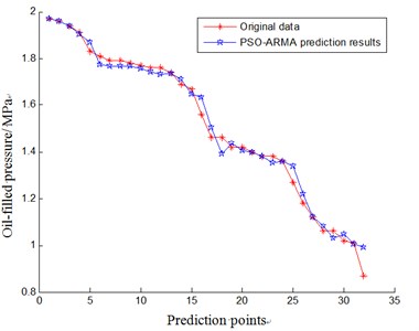
Fig. 3The comparison of aero-generator condition trend prediction based on PSO-ARMA and ARMA
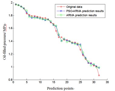
Table 1The comparison of prediction error between PSO-ARMA and ARMA
Prediction model | Prediction error | ||
ARMA model | 2 | 6 | 0.0264 |
PSO-ARMA model | 4 | 2 | 0.0203 |
6.2. Research on aero-generator life prediction based on PSO-LSSVM
Similar with the prediction thought for condition and trend of aero-generator with PSO-ARMA model, firstly, PSO parameters need to be initialized. To set initialization value of each parameter of PSO-LSSVM model as: 100, 60, 2, 2, 2. In addition, in this paper, we initialize the parameter of PSO-LSSVM as the regularization: 40; kernel function is selected as Radial Basis Function(RBF), and the wide of kernel is: 7.
After initialization, we use PSO-LSSVM model to solve parameters. When the mean square deviation of prediction result is zero or the iterative times are 100, the process of algorithm is over. Then we can get the optimal parameters, they are: 65.0281, 5.4402. Afterwards, we bring the optimal parameter into LSSVM and reconstruct regression model with test samples. At last, we can get the condition parameters of aero-generator: the trend prediction of oil-filled pressure. Taking 32 prediction values and target values into connect curve, we can predict the condition and trend of aero-generator in certain period of time. The prediction results are shown in Fig. 4.
To demonstrate that the accuracy of PSO-LSSVM is higher than that of LSSVM, we plot original data of oil injection pressure, prediction results based on PSO-LLSVM and prediction results based on LSSVM in a same figure, which is shown in Fig. 5.
Fig. 4The result of aero-generator condition trend prediction based on PSO-LSSVM
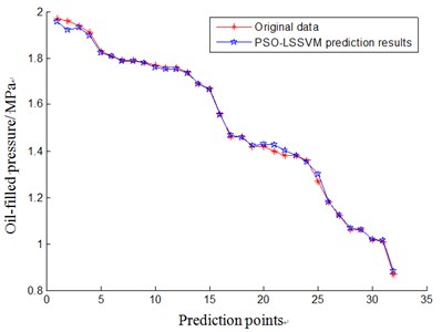
Fig. 5The comparison of aero-generator condition trend prediction based on PSO-LSSVM and LSSVM
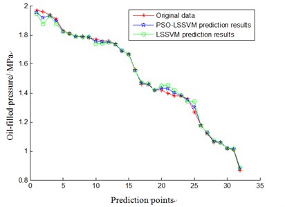
By calculating and anglicizing the model before and after optimization trend predictor, we can get prediction error of the PSO-LSSVM and LSSVM, which is shown in Table 2.
Table 2 shows the contrastive data of average prediction error after some tests. The data shows that prediction relative error is 1.69 % with LSSVM model, while the error is 0.83 % with PSO-LSSVM model. Researches demonstrate that the result is more exact with PSO-LSSVM model to predict condition and trend of aero-generator.
Table 2The comparison of prediction error between PSO-LSSVM and LSSVM
Prediction model | Prediction error | ||
LSSVM model | 40 | 7 | 0.0169 |
PSO-LSSVM model | 65.0281 | 5.4402 | 0.0083 |
7. Research on aero-generator condition trend prediction based on fuzzy integral fusion
In this paper, we use PSO-ARMA and PSO-LLSVM to predict and analyze the trend of oil-filled pressure respectively. The result shows that there are large differences between PSO-ARMA and PSO-LSSVM. To realize a comprehensive and accurate decision, we apply fuzzy integral algorithm to make a decision level fusion of prediction results of PSO-ARMA and PSO-LSSVM [24]. When we make the fusion, we need to know the fuzzy density. Here, according to the prediction precision of two models, we define the decision importance as the fuzzy density, and it is feasible. We can solve with Eq. (3), bring it into Eq. (2), we can get the fuzzy measure. Next, we use Eq. (4) to fuse the information, the error after fusion is only 0.79 %. So, we can see that the error after fusion is smaller than that before fusion. Which as shown in Table 3.
From Table 3, we can see the error of life prediction is reduced and the accuracy is raised after fusing with Fuzzy integral. The result can reflect the remaining life information of aero-generator better.
Table 3The comparison of forecast errors between before and after fusion
Prediction algorithm | PSO-ARMA model | PSO-LSSVM model | Fuzzy integral fusion |
Prediction error | 2.03 % | 0.83 % | 0.79 % |
8. Conclusions
1) Two optimized models of the PSO-ARMA and the PSO-LSSVM are presented in this paper. We use those two new models to predict the change of the air generator’s condition trend. The condition trend prediction error of PSO-ARMA which is 2.03 is lower than that of ARMA (2, 6) which is 2.64 %. The condition trend prediction error of PSO-LSSVM which is 0.83 % is much lower than that of LSSVM which is 1.69 %. The above results demonstrate that PSO can improve the prediction performance more effectively.
2) The prediction results of PSO-ARMA and PSO-LSSVM are fused using Fuzzy Integral Fusion Algorithm and the prediction error after fusion is only 0.79 %. The error is smaller than that of each presented model. It can reflect the trend of oil-filled pressure better, and it can be supplied for preventive maintenance. Moreover, the presented methods are also feasible in condition trend prediction of other complex systems and have a broad application prospects.
References
-
Ouyang Wen, Xie Kaigui, Wang Xiaobo, Feng Yi, Hu Bo, Cao Kan Modeling of generation system reliability variation with reliability parameters and electrical parameters. Electric Power Automation Equipment, Vol. 29, Issue 4, 2009, p. 41-45.
-
Wang Hongjun, Xu Xiaoli, Zhang Jianmin Support vector machine condition trend prediction technology. Mechanical Science and Technology, Vol. 25, Issue 4, 2006, p. 379-381.
-
Yu Ren, Zhang Yonggang, Ye Luqing, Li Zhaohui The analysis and design method of maintenance system in intelligent control-maintenance-technical management system (ICMMS) and ITS application. Proceedings of the CSEE, Vol. 21, Issue 4, 2001, p. 60-65.
-
Xiong Tiehua, Liang Shuguo, Zou Lianghao Wind loading identification of transmission towers based-on wind tunnel tests of full aero-elastic model. Journal of Building Structures, Vol. 31, Issue 10, 2010, p. 48-54.
-
Chen Guo Forecasting engine performance trend by using structure self-adaptive neural network. Acta Aeronautica ET Astronautica Sinica, Vol. 28, Issue 3, 2007, p. 535-539.
-
Xu Feng, Wang Zhifang, Wang Baosheng Research on AR model applied to forecast trend of vibration signals. Journal of Tsinghua University (Science and Technology), Vol. 39, Issue 4, 1999, p. 57-59.
-
Vapnik V. N. An overview of statistical learning theory. IEEE Transactions on Neural Networks, Vol. 10, Issue 5, 1999, p. 988-999.
-
Smola A. J., Scholkopf B. A tutorial on support vector regression. Statistics and Computing, Vol. 14, Issue 3, 2004, p. 199-222.
-
Zhu Qibing, Liu Jie, Li Yungong, Wen Bangchun Study on noise reduction in singular value decomposition based on structural risk minimization. Journal of Vibration Engineering, Vol. 18, Issue 2, 2005, p. 204-207.
-
Ji Xunsheng Short-term power load forecasting on partial least square support vector machine. Power System Protection and Control, Vol. 38, Issue 23, 2010, p. 55-59.
-
Huan Hongjiang, Gong Ningsheng, Hu Bin Application of modified BP neural network in traffic flow forecasts. Microelectronics and Computer, Vol. 27, Issue 1, 2010, p. 106-108.
-
Lei Xiujuan, Shi Zhongke, Zhou Yipeng Evolvement of particle swarm optimization and its combination strategy. Computer Engineering and Applications, Vol. 43, Issue 7, 2007, p. 90-92.
-
Luo Hang, Huang Jianguo, Long Bing, Wang Houjun Searching ARMA model parameters MLE-Based by applying PSO algorithm. Journal of University of Electronic Science and Technology of China, Vol. 39, Issue 1, 2010, p. 65-68.
-
Zhao Chunguang Research on Applications of Fuzzy Integral in Multiple Analysis. Northeastern University, Shenyang, 2008.
-
Kennedy J., Eberhart R. C. Particle swarm optimization. Proceedings IEEE International Conference on Neural Networks, 1995, p. 1942-1948.
-
Shi Yuhui, Eberhart R. C. Parameter selection in particle swarm optimization. Springer Verlag, Vol. 1447, 1998, p. 591-600.
-
Niu Ditao, Wang Qinglin, Dong Zhenping Probability model and statistical parameters of resistance for existing structure. Journal of Xi’an University of Architecture and Technology, Vol. 29, Issue 4, 1997, p. 355-359.
-
Han Luyue, Du Xingjian Modeling and prediction of time series based on Matlab. Computer Simulation, Vol. 22, Issue 4, 2005, p. 105-107.
-
Zhao Shutao, Pan Lianling, Li Baoshu Fault diagnosis and trend forecast of transformer based on acoustic recognition. The 3rd International Conference on Deregulation and Restructuring and Power Technologies, 2008, p. 1371-1374.
-
He Shuyuan Applied Time Series Analysis. Peking University Press, Beijing, 2003.
-
Mohammadi Kourosh, Eslami H. R., Kahawita Rene Parameter estimation of an ARMA model for river flow forecasting using goal programming. Journal of Hydrology, Vol. 331, Issues 1-2, 2006, p. 293-299.
-
Xie Zhipeng Positive definite kernel in support vector machine (SVM). Transactions of Nanjing University of Aeronautics and Astronautics, Vol. 26, Issue 2, 2009, p. 114-121.
-
Liu Donghui, Bian Jianpeng, Fu Ping, Liu Zhiqing Study on the choice optimum parameters of support vector machine. Journal of Hebei University of Science and Technology, Vol. 30, Issue 1, 2009, p. 58-61.
-
Wang Yan, Zhang Shuhong, Qu Yili Fault diagnosis method based on fuzzy integral decision level fusion. Techniques of Automation and Applications, Vol. 5, 2001, p. 14-16.
About this article

This work is supported by the Aeronautic Science Foundation of China (ID20153354005, ID20163354004), the Base of Defense Scientific Research Projects of China (IDZ052012B002) and the Natural Science Foundation of Liaoning Province (ID2014024003).
Jianguo Cui mainly design and improve the algorithm. Wei Zheng and Liying Jiang major editing and improvement program. Huihua Li conclusions are verified. Mingyue Yu design overscheme.
