Operating state prediction for wind turbine generator bearing based on ULSSVM and QPSO

1. Introduction

Wind turbine has been in a rapid growth mode since the 20th century. This rapid growth also affects the performance of wind turbines. The generator is one of the key components of the wind turbine [1]. Bearings are used in generators. The operating state of the bearing is not only related to the normal operation of the generator, but also related to the stable operation of the wind turbine [2]. The damaged bearings are often the leading cause of machine downtime and huge economic loss [3, 4]. Effectively predicting the operating status of the wind turbine generator can reduce downtime and economic loss.

Data prediction is significant for operating state prediction. Least squares support vector machine (LSSVM) is a commonly used method in data prediction [5-7]. However, this method often only considers the trend of a single characteristic parameter with time and does not consider the interaction between various characteristic parameters. In the prediction process, there are often correlations among various characteristic parameters. The change of a certain characteristic parameter will reflect or affect the change of other characteristic parameters to a certain extent. Aiming at this problem, a prediction method based united least squares support vector machine (ULSSVM) is proposed. ULSSVM method combines time least squares support vector machine (TLSSVM) model and space least squares support vector machine (SLSSVM) model. The TLSSVM model is established based on the law of characteristic parameters changing with time. The SLSSVM model is established based on the relationship between the characteristic parameters. In the training phase of the model, the original data sequence is used as input. The TLSSVM model and the SLSSVM model are obtained separately through training. The weight value of each model is also essential. Then, the weight values need to be determined. The TLSSVM model and the SLSSVM model are combined. The ULSSVM prediction model is obtained. If the weight values are obtained through experience, it will produce great subjectivity and uncertainty. Dempster-Shafer (D-S) has advantages in dealing with uncertainties caused by unknowns. It does not require prior probability and is easy to calculate. Therefore, it is widely used in data information fusion processing [8-10]. The traditional D-S theory has great limitations when dealing with conflicting information. The improved D-S theory can avoid this problem.

Parameter selection directly affects the prediction effect of LSSVM. In order to obtain the optimal parameters, the optimization method is generally used to optimize LSSVM parameters [11]. [12] utilized an adaptive cuckoo search method to optimize the kernel parameter and the penalty parameter of the LSSVM model. Compared with no parameter optimization, the mean absolute percentage error is reduced by nearly 30 %. Recently, there are many methods for LSSVM parameter optimization, such as particle swarm optimization (PSO), improved PSO, hybrid particle swarm optimization, and niche particle swarm optimization [13-16]. PSO method is suitable for LSSVM parameter optimization and is widely used. It is easy to implement, but it is slow for global convergence. Quantum particle swarm optimization (QPSO) is proposed based on PSO [17]. This model assumes that particles have quantum behavioral characteristics. The algorithm can search in the entire feasible area. So that the global search ability of QPSO is better than PSO.

In this research, an operating state prediction method for wind turbine bearings based on united LSSVM and QPSO is proposed. United LSSVM includes time LSSVM model and space LSSVM model. QPSO is used for parameter optimization of the models. The weights of time LSSVM and space LSSVM are determined by the improved D-S theory. The proposed method can improve the accuracy of the predicted values. The mean absolute error, the mean absolute percentage error, and the root mean squared error can be reduced. A case study shows that the prediction results based on this method can realize the prediction of the operating state of the wind turbine bearing.

2. Basic theory

3. Proposed parameter prediction scheme

If the time least squares support vector machine is used to predict the characteristic parameter, the historical test data of this parameter is used to predict the value of the parameter at a certain time in the future. The characteristic parameter set is expressed as $V=\left\{v_1,v_2,\dots ,v_n\right\}$. Specifically, part of the test data $x_{i,t},x_{i,t-1},...,x_{i,t-m+1}$ of the characteristic parameter $v_i$ before time $t$ is obtained. $m$ is the preset embedding dimension. Then the LSSVM is used to get the fitting function $f_1$. The value of the characteristic parameter $v_i$ at time $t+1$ is predicted by $f_1$. The interrelation is depicted by the term:

Traditional prediction models only consider the trend of the characteristic parameters over time. It cannot reflect the mutual influence and interrelationship among various characteristic parameters. In practical applications, the change of one parameter will affect the change of other parameters. In complex equipment systems, the correlation between different parameters cannot be ignored. In order to improve the prediction accuracy, the correlation between the parameters must be fully considered. Therefore, the traditional LSSVM modeling process needs to be improved. Incorporating the correlation between the parameters, a space LSSVM is proposed. Specifically, the test data $x_{1,t},\mathrm{}{x}_{2,t},\dots ,x_{n,t}$ of the characteristic parameter set $V$ at time $t$ is obtained. Then the space LSSVM is used to get the fitting function $f_2$. The value of parameter $v_i$ at time $t+1$ is predicted by $f_2$. The interrelation is depicted by the term:

TLSSVM prediction model considers the effect of time on the characteristic parameters. SLSSVM prediction model considers the interaction between various parameters. In order to improve the prediction accuracy, these two prediction models need to be fused reasonably. ULSSVM is built as a modified LSSVM.

When using time LSSVM, the predicted value of the characteristic parameter $v_i$ at time $t+1$ is expressed as ${x^1}_{i,t+1}$. When using space LSSVM, the predicted value of the characteristic parameter $v_i$ at time $t+1$ is expressed as ${x^2}_{i,t+1}$. Based on the above two predicted values of ${x^1}_{i,t+1}$ and ${x^2}_{i,t+1}$, a combined function can be constructed:

The weighted form of the combined function is obtained by the following:

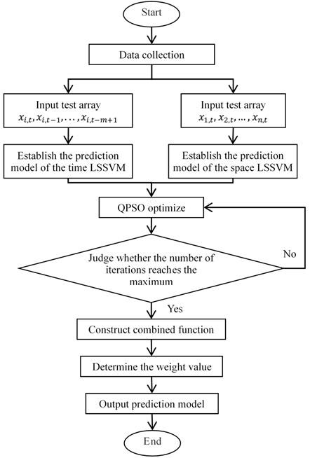
where ${{\omega }^1}_{i,t+1}$ is the weight of the TLSSVM prediction model. ${{\omega }^2}_{i,t+1}$ is the weight of the SLSSVM prediction model. Improved D-S theory is used to obtain the weight values. Select samples from test samples for evidence fusion analysis. Samples with close working condition data are preferred. A flowchart of the proposed parameter prediction scheme is shown in Fig. 1.

Take the prediction process of a certain characteristic parameter $v_i$ as an example. The concrete steps of the parameter prediction scheme based on ULSSVM, QPSO and improved D-S are as follows:

(1) The test data of the characteristic parameter $v_i$ in a period of time before $t$ is collected, and the collection results are represented by $x_{i,t},x_{i,t-1},...,x_{i,t-m+1}$. TLSSVM is used to obtain the fitting map $f_1$. $f_1$ is used to predict the value of $v_i$ at $t+1$ by Eq. (12). QPSO algorithm is used to optimize the kernel parameter and the penalty parameter of the LSSVM model. The prediction result is represented by ${x^1}_{i,t+1}$.

(2) Collect the test data of all characteristic parameters at time $t$. The collection results are $x_{1,t},x_{2,t},\dots ,x_{n,t}$. SLSSVM is used to obtain the fitting map $f_2$. $f_2$ is used to predict the value of $v_i$ at $t+1$ by Eq. (13). QPSO algorithm is used to optimize the kernel parameter and the penalty parameter of the LSSVM model. The prediction result is represented by ${x^2}_{i,t+1}$.

(3) The predicted value ${x^1}_{i,t+1}$ and the predicted value ${x^2}_{i,t+1}$ are used to construct a combined function in the form of Eq. (15).

(4) The weight values ${{\omega }^1}_{i,t+1}$ and ${{\omega }^2}_{i,t+1}$ in Eq. (15) are determined according to the actual measured value of the characteristic parameter $v_i$ at $t+1$.

(5) According to the calculation results, the final prediction model is determined.

The final prediction model will be used to predict the value of $v_i$ at time $t+2$.

Fig. 1Flowchart of the proposed parameter prediction scheme

4. Bearing parameter prediction based on ULSSVM

In order to verify the effectiveness of the proposed parameter prediction method, it is used for parameter prediction of bearing vibration signals and compared with actual measured values.

4.1. Data acquisition

Vibration signals of rotating machinery often contain rich operating status information [22-25]. Collect a set of bearing vibration signals under working conditions every 15 days. A total of 205 sets of vibration signal test data have been recorded. The sampling frequency is 20000 Hz, and the number of sampling points is 20480. 1-170 sets of vibration signal test data are used for training and learning. 171-205 sets of vibration signal test data are used for prediction and comparison.

The original data is difficult to reflect the operating state of the bearing. It is necessary to extract the characteristic parameters representing the operating state [26, 27]. There are many parameters that can be used to describe the operating state of the bearing [28, 29]. According to the existing research results of the bearing state prediction, 10 characteristic parameters are selected to represent the operating state of the bearing. The 10 parameters are mean value, rectified mean value, variance, root mean square (RMS), kurtosis, form factor, peak-to-average ratio (PAR), kurtosis factor, impulse factor and margin factor. These 10 parameters form a matrix $V=\left\{v_1,v_2,v_3,v_4,v_5,v_6,v_7,v_8,v_9,v_{10}\right\}$. $v_1$ is the mean value. $v_2$ is the rectified mean value. $v_3$ is the variance. $v_4$ is RMS. $v_5$ is the kurtosis. $v_6$ is the form factor. $v_7$ is PAR. $v_8$ is the kurtosis factor. $v_9$ is the impulse factor. $v_{10}$ is the margin factor.

The mean value is the average value of all signal amplitudes. It can be expressed as:

16

$\mu =\frac{{\sum }_{i=1}^n{x}_i}{n},$

where $\mu$ is the mean value. $n$ is the number of sampling points. $x_i$ is the amplitude of the $i$-th sampling point.

The rectified mean value is the average of the absolute values of all amplitudes. It can be expressed as:

17

${\mu }_{av}=\frac{{\sum }_{i=1}^n\left|x_i\right|}{n}.$

The variance is the average of the square of the difference between the amplitude of each signal and the average of all signal amplitudes. It represents the dynamic component of signal energy. It can be expressed as:

18

${\sigma }^2=\frac{1}{n}{\sum }_{i=1}^n{\left[x_i-\mu \right]}^2.$

The RMS calculation process is to sum the squares of all signal amplitudes and take their average. Then take the square root of the calculation result. The root mean square is also called the effective value. It can be expressed as:

19

$X_{rms}=\sqrt{\frac{{\sum }_{i=1}^n{x_i}^2}{n}}.$

The kurtosis is used to describe the sharpness of the waveform. It can be expressed as:

20

$K=\frac{E{\left[x_i-\mu \right]}^4}{X_{rms}^4}.$

The form factor is the ratio of the RMS to the rectified mean value. It can be expressed as:

21

$S=\frac{X_{rms}}{{\mu }_{\text{av}}}.$

PAR is the ratio of the peak value to the RMS. It represents the extreme degree of peaks in the waveform. It can be expressed as:

22

$C=\frac{X_{peak}}{X_{rms}},$

where $X_{peak}$ is the peak value of the signal.

The kurtosis factor is used to describe the smoothness of the waveform. It is the distribution of variables. It can be expressed as:

23

$K_F=\frac{{\sum }_{i=1}^n{x_i}^2}{n{X}_{rms}^4}.$

The impulse factor is the ratio of the peak value to the rectified mean value. The difference between impulse factor and PAR is the denominator. For the same group of signals, the rectified mean value must be less than its effective value, so the impulse factor must be greater than the PAR. The impulse factor can be expressed as:

24

$I=\frac{X_{peak}}{{\mu }_{\text{av}}}.$

The margin factor is the ratio of the peak value to the square root amplitude. It is similar to PAR. The square root amplitude and the RMS are corresponding. It can be expressed as:

25

$CL=\frac{X_{peak}}{{\left(\frac{1}{n}{\sum }_{i=1}^n\sqrt{\left|x_i\right|}\right)}^2}.$

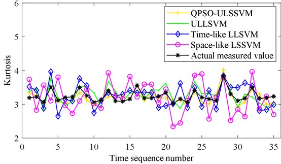
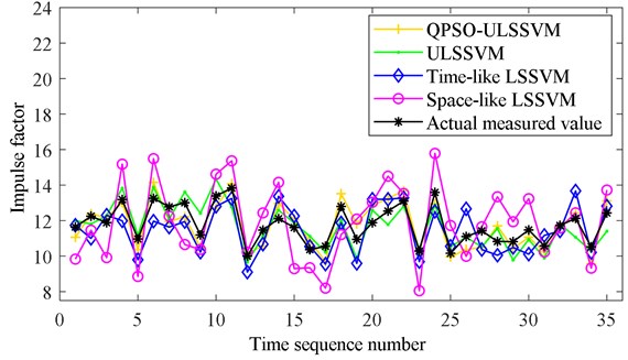
All state characteristic parameters of 205 sets of test data are calculated separately, including mean value, rectified mean value, variance, RMS, kurtosis, form factor, PAR, kurtosis factor, impulse factor, and margin factor. To reduce the complexity of the calculation, two characteristic parameters are selected as the prediction parameters, including the kurtosis and the impulse factor. The calculation results of the kurtosis are shown in Fig. 2(a). The calculation results of the impulse factor are shown in Fig. 2(b). It shows that the change regularities of the characteristic parameters are complicated.

Fig. 2Characteristic parameters of bearing vibration signal: a) the kurtosis and b) the impulse factor

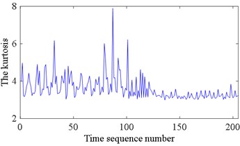
a)

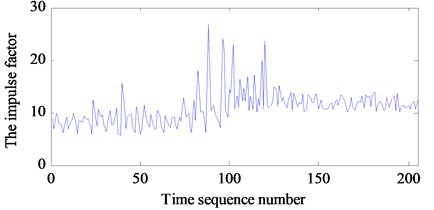
b)

4.2. Comparison of prediction methods

To evaluate the effectiveness and exhibit the superiority of QPSO ULSSVM algorithm in the prediction of characteristic parameters, the kurtosis and the impulse factor are predicted. TLSSVM, SLSSVM, ULSSVM and QPSO ULSSVM are used to predict the characteristic parameters separately. The mean absolute error ${\sigma }_{MAE}$, the mean absolute percentage error ${\sigma }_{MAPE}$, and the root mean squared error ${\sigma }_{RMSE}$ are selected to evaluate these four methods. The expressions are as follows:

26

${\sigma }_{MAE}=\frac{1}{n}{\sum }_{i\text{=1}}^n\left|\widehat{y}\left(i\right)-y\left(i\right)\right|,$

27

${\sigma }_{MAPE}=\frac{1}{n}{\sum }_{i\text{=1}}^n\left|\frac{\widehat{y}\left(i\right)-y\left(i\right)}{y\left(i\right)}\right|\times \text{100 \%},$

28

${\sigma }_{RMSE}=\sqrt{\frac{1}{n}{\sum }_{i\text{=1}}^n{\left[\widehat{y}\left(i\right)-y\left(i\right)\right]}^2},$

where $n$ is the number of samples. $y\left(i\right)$ is the measured value. $\widehat{y}\left(i\right)$ is the prediction value.

TLSSVM is used to predict the kurtosis. The kurtosis $v_1$ of 171-205 data sets are predicted based on 1-170 data sets. ${\sigma }_{MAE}$, ${\sigma }_{MAPE}$, and ${\sigma }_{RMSE}$ are calculated based on TLSSVM predicted results and measured results.

SLSSVM is used to predict the kurtosis. The kurtosis $v_1$ of the 171-th data set is predicted based on all state characteristic parameters of the 170-th data set. $v_1$ of the 172-th data set is predicted based on all state characteristic parameters of the 171-th data set. $v_1$ of the $n$-th data set is predicted based on all state characteristic parameters of the ($n-1$)th data set. 171-205 data sets are predicted by using the same method. ${\sigma }_{MAE}$, ${\sigma }_{MAPE}$, and ${\sigma }_{RMSE}$ are calculated based on SLSSVM predicted results and measured results.

ULSSVM is used to predict the kurtosis. The kurtosis $v_1$ of 171-205 data sets are predicted based on 171-205 prediction results of TLSSVM and SLSSVM, respectively. Weight values are determined by the improved D-S theory. ULSSVM predicted results are output based on weight values, TLSSVM prediction results, and SLSSVM prediction results. ${\sigma }_{MAE}$, ${\sigma }_{MAPE}$, and ${\sigma }_{RMSE}$ are calculated based on ULSSVM predicted results and measured results.

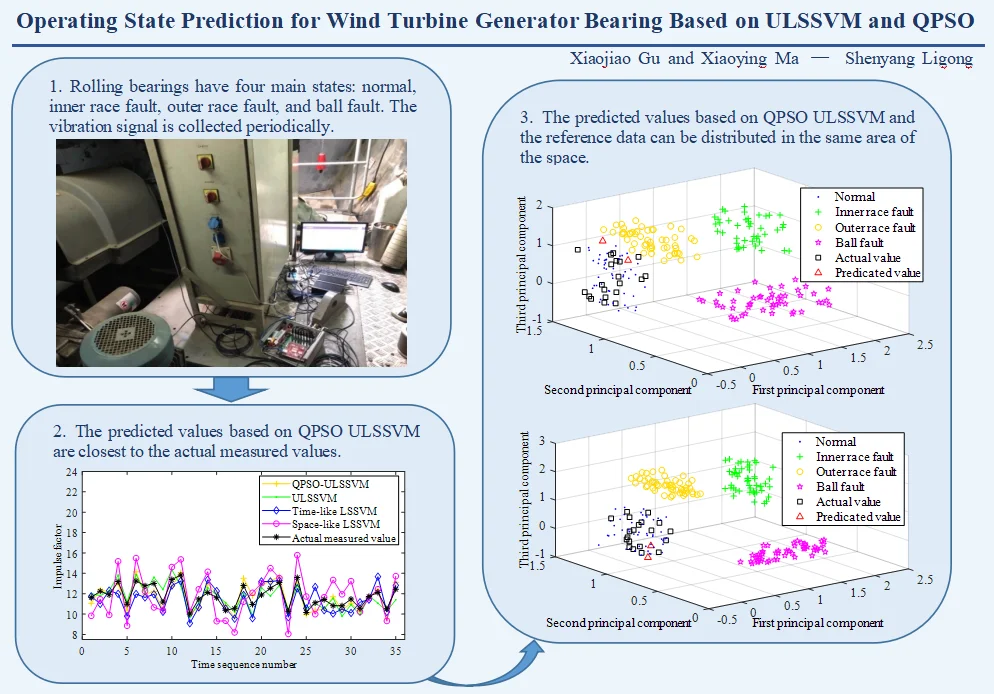
QPSO ULSSVM is used to predict the kurtosis. TLSSVM and SLSSVM are optimized by QPSO. The kurtosis $v_1$ of 171-205 data sets are predicted based on optimized TLSSVM and SLSSVM, respectively. Then the weight values are calculated and the prediction results are output. ${\sigma }_{MAE}$, ${\sigma }_{MAPE}$, and ${\sigma }_{RMSE}$ are calculated based on QPSO ULSSVM prediction results and measured results. The impulse factor $v_2$ is predicted by using the same method. The prediction results are shown in Fig. 3. It shows that the predicted values based on QPSO ULSSVM are closest to the actual measured values.

Table 1Evaluation values of the prediction results

Parameter	Method	Evaluation index
		${\sigma }_{MAE}$	${\sigma }_{MAPE}$	${\sigma }_{RMSE}$
Kurtosis	TLSSVM	0.2331	0.0725	1.1245
	SLSSVM	0.3791	0.1175	1.8344
	ULSSVM	0.1860	0.0576	0.8488
	QPSO ULSSVM	0.1143	0.0351	0.5756
Impulse factor	TLSSVM	0.8372	0.0712	3.9071
	SLSSVM	1.3896	0.1183	6.5391
	ULSSVM	0.5981	0.0505	2.8265
	QPSO ULSSVM	0.5718	0.0487	2.6752

The evaluation values of the prediction results are shown in Table 1, which can show that all of the four prediction methods can predict the characteristic parameters. This demonstrates that the bearing characteristic parameters have specific variation trend and could be predicted. Furthermore, the method based on QPSO ULSSVM yields the best accuracy, significantly higher than TLSSVM, SLSSVM, and ULSSVM. This will provide help for operating state recognition.

Fig. 3Predicted results of characteristic parameters: a) kurtosis and b) impulse factor

a)

b)

5. Case study

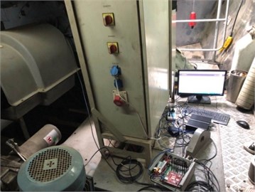
To verify the proposed method, bearing fault prediction is implemented. The vibration signal collection of the generator bearing is shown in Fig. 4. It is collected in the wind turbine nacelle. The acceleration sensor is installed on the bearing saddle. The vibration signal is collected periodically. Rolling bearings have four main states: normal, inner race fault, outer race fault, and ball fault. Collect 50 sets of vibration data for bearings of the same model in these four states, respectively. These data are called reference data. 10 characteristic parameters of each set of vibration data are calculated, respectively. The results of each state can be formed into a 50×10 matrix. This matrix is used as the reference matrix.

The vibration data of the same model bearing to be predicted is collected. Data is collected once a week. The total number of the collections is 20. The group number of each set of data is arranged from small to large according to time. These data are called test data. 10 characteristic parameters of each set of vibration data are calculated, respectively. The order of the 10 characteristic parameters is consistent with the reference matrix. Set the sequence number of the characteristic parameters: mean value is 1, rectified mean value is 2, variance is 3, RMS is 4, kurtosis is 5, form factor is 6, PAR is 7, kurtosis factor is 8, impulse factor is 9, margin factor is 10. Combine all calculation results into a matrix. The number of the row represents the time. The number of the column represents the sequence number of the characteristic parameter. It can be expressed as:

Fig. 4Data acquisition test device

QPSO ULSSVM is used to predict the characteristic parameters of the next moment. Take the mean value as an example. The mean values of 1-19 sets of test data are extracted as Eq. (30). The 10 characteristic parameters of 19-th set of test data are extracted as Eq. (31). LSSVM is used to fit the fitting function $f_1$. $f_1$ is required to meet Eq. (32). LSSVM is used to fit the fitting function $f_2$. $f_2$ is required to meet Eq. (33). The weight values of $f_1$ and $f_2$ are determined by using improved D-S theory. The weight values are ${\omega }_{\mathrm{1,21}}^1$ and ${\omega }_{\mathrm{1,21}}^2$, respectively. The mean value at the next moment $x_{\mathrm{21,1}}$ is predicted by Eq. (34). The other 9 parameters are rectified mean value, variance, RMS, kurtosis, form factor, PAR, kurtosis factor, impulse factor, and margin factor. The prediction method is the same as that of the mean value. The 10 characteristic parameters are predicted by using QPSO ULSSVM:

The parameter reference matrices of the four states are subjected to Laplacian eigenmaps (LE) dimensionality reduction processing. The feature vectors obtained by dimensionality reduction are fused. The feature vectors of the first three dimensions are extracted. The three-dimensional visualization of the reference matrix is obtained as shown in Fig. 5. The four states are well distinguished. The prediction results of 21-th set of data and the parameter reference matrices form a new matrix. This new matrix is reduced in dimension by LE. The feature vectors are fused and the first three dimensions of the feature vectors are extracted. The calculation result is expressed in the form of a three-dimensional image, as shown in Fig. 6. The prediction data and the normal state data are distributed in the same area of the space. The prediction result is that the bearing state is normal at the next moment. The bearing is working normally after a week.

Fig. 5Three-dimensional classification diagram of the four states

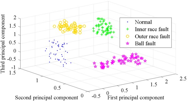
Fig. 6Three-dimensional classification diagram of the prediction result based on QPSO ULSSVM

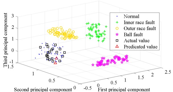
Fig. 7Three-dimensional classification diagram of the prediction result based on LSSVM

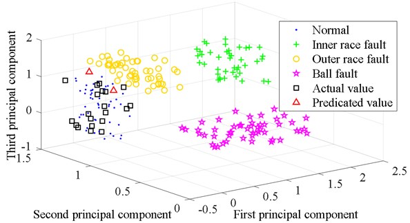
As a comparison, the characteristic parameters prediction method uses TLSSVM. The 10 characteristic parameters of 21-th set of data are predicted by using traditional TLSSVM. The prediction results and the parameter reference matrices form a new matrix. This new matrix is also reduced in dimension by LE. The first three feature vectors are extracted. The calculation result is expressed in the form of a three-dimensional image, as shown in Fig. 7. The prediction data, the outer race fault data, and the normal state data are partially overlapped. The result is not certain. This shows that the accuracy of state parameter prediction is related to generator bearing’s operating state prediction. QPSO ULSSVM improves the accuracy of characteristic parameters prediction. The realization of the generator bearing’s operating state prediction is based on QPSO ULSSVM.

6. Conclusions

In this paper, ULSSVM and QPSO is used to predict the operating status of the wind turbine bearing. The observations and conclusions of the study are summarized as follows:

1) ULSSVM, a novel parameter prediction method, is proposed to effectively predict the operating state parameters. The results show that the new method is better than the TLSSVM and SLSSVM methods.

2) ULSSVM combines the time LSSVM and the space LSSVM. Improved D-S method is used to determine the weight of each model. It helps ULSSVM achieve better results in the parameter prediction of wind turbine bearing.

3) The novel strategy of utilizing combined ULSSVM and QPSO to parameter prediction in wind turbine bearing is developed, and the algorithm is proved reliable to predict the working state of wind turbine bearing. It was provided an effectual way for the operating state prediction of wind turbine bearing to combine ULSSVM and QPSO.